Introduction¶

Getting started¶

Before you start moving around in Yade, you should have some prior knowledge.

Basics of command line in your Linux system are necessary for running yade. Look on the web for tutorials.
Python language; we recommend the official Python tutorial. Reading further documents on the topic, such as Dive into Python will certainly not hurt either.

You are advised to try all commands described yourself. Don’t be afraid to experiment.

Hint

Sometimes reading this documentation in a .pdf format can be more comfortable. For example in okular pdf viewer clicking links is faster than a page refresh in the web browser and to go back press the shortcut Alt Shift ←. To try it have a look at the inheritance graph of PartialEngine then go back.

Starting yade¶

Yade is being run primarily from terminal; the name of command is yade. [1] (In case you did not install from package, you might need to give specific path to the command [2]):

$ yade
Welcome to Yade
TCP python prompt on localhost:9001, auth cookie `sdksuy'
TCP info provider on localhost:21000
[[ ^L clears screen, ^U kills line. F12 controller, F11 3d view, F10 both, F9 generator, F8 plot. ]]
Yade [1]:

These initial lines give you some information about

some information for Remote control, which you are unlikely to need now;
basic help for the command-line that just appeared (Yade [1]:).

Type quit(), exit() or simply press ^D (^ is a commonly used written shortcut for pressing the Ctrl key, so here ^D means Ctrl D) to quit Yade.

The command-line is ipython, python shell with enhanced interactive capabilities; it features persistent history (remembers commands from your last sessions), searching and so on. See ipython’s documentation for more details.

Typically, you will not type Yade commands by hand, but use scripts, python programs describing and running your simulations. Let us take the most simple script that will just print “Hello world!”:

print("Hello world!")

Saving such script as hello.py, it can be given as argument to Yade:

$ yade hello.py
Welcome to Yade
TCP python prompt on localhost:9001, auth cookie `askcsu'
TCP info provider on localhost:21000
Running script hello.py                                           ## the script is being run
Hello world!                                                      ## output from the script
[[ ^L clears screen, ^U kills line. F12 controller, F11 3d view, F10 both, F9 generator, F8 plot. ]]
Yade [1]:

Yade will run the script and then drop to the command-line again. [3] If you want Yade to quit immediately after running the script, use the -x switch:

$ yade -x script.py

There is more command-line options than just -x, run yade -h to see all of them.

Options:

-v, --version show program’s version number and exit

-h, --help show this help message and exit

-j THREADS, --threads=THREADS

Number of OpenMP threads to run; defaults to 1. Equivalent to setting OMP_NUM_THREADS environment variable.

--cores=CORES Set number of OpenMP threads (as –threads) and in addition set affinity of threads to the cores given.

--update Update deprecated class names in given script(s) using text search & replace. Changed files will be backed up with ~ suffix. Exit when done without running any simulation.

--nice=NICE Increase nice level (i.e. decrease priority) by given number.

-x Exit when the script finishes

-f Set logging verbosity, default is -f3 (yade.log.WARN) for all classes

-n Run without graphical interface (equivalent to unsetting the DISPLAY environment variable)

--test Run regression test suite and exit; the exists status is 0 if all tests pass, 1 if a test fails and 2 for an unspecified exception.

--check Run a series of user-defined check tests as described in scripts/checks-and-tests/checks/README and Regression tests

--performance Starts a test to measure the productivity.

--stdperformance

Starts a standardized test to measure the productivity, which will keep retrying to run the benchmark until standard deviation of the performance is below 1%. A common type of simulation is done: the spheres fall down in a box and are given enough time to settle in there. Note: better to use this with argument -j THREADS (explained above).

--quickperformance

Starts a quick test to measure the productivity. Same as above, but only two short runs are performed, without the attempts to find the computer performance with small error.

--no-gdb Do not show backtrace when yade crashes (only effective with –debug) [4].

Footnotes

[1] The executable name can carry a suffix, such as version number (yade-0.20), depending on compilation options. Packaged versions on Debian systems always provide the plain yade alias, by default pointing to latest stable version (or latest snapshot, if no stable version is installed). You can use update-alternatives to change this.

[2]

In general, Unix shell (command line) has environment variable PATH defined, which determines directories searched for executable files if you give name of the file without path. Typically, $PATH contains /usr/bin/, /usr/local/bin, /bin and others; you can inspect your PATH by typing echo $PATH in the shell (directories are separated by :).

If Yade executable is not in directory contained in PATH, you have to specify it by hand, i.e. by typing the path in front of the filename, such as in /home/user/bin/yade and similar. You can also navigate to the directory itself (cd ~/bin/yade, where ~ is replaced by your home directory automatically) and type ./yade then (the . is the current directory, so ./ specifies that the file is to be found in the current directory).

To save typing, you can add the directory where Yade is installed to your PATH, typically by editing ~/.profile (in normal cases automatically executed when shell starts up) file adding line like export PATH=/home/user/bin:$PATH. You can also define an alias by saying alias yade="/home/users/bin/yade" in that file.

Details depend on what shell you use (bash, zsh, tcsh, …) and you will find more information in introductory material on Linux/Unix.

[3]

Plain Python interpreter exits once it finishes running the script. The reason why Yade does the contrary is that most of the time script only sets up simulation and lets it run; since computation typically runs in background thread, the script is technically finished, but the computation is running.

[4]	On some linux systems stack trace will produce `Operation not permitted` error. See debugging section for solution.

Quick inline help¶

All of functions callable from ipython shell have a quickly accessible help by appending ? to the function name, or calling help(…) command on them:

Yade [1]: O.run?
Docstring:
run( (Omega)arg1 [, (int)nSteps=-1 [, (bool)wait=False]]) -> None :
    Run the simulation. *nSteps* how many steps to run, then stop (if positive); *wait* will cause not returning to python until simulation will have stopped.
Type:      method


Yade [2]: help(O.pause)
Help on method pause:

pause(...) method of yade.wrapper.Omega instance
    pause( (Omega)arg1) -> None :
        Stop simulation execution. (May be called from within the loop, and it will stop after the current step).

A quick way to discover available functions is by using the tab-completion mechanism, e.g. type O. then press tab.

Creating simulation¶

To create simulation, one can either use a specialized class of type FileGenerator to create full scene, possibly receiving some parameters. Generators are written in C++ and their role is limited to well-defined scenarios. For instance, to create triaxial test scene:

Yade [3]: TriaxialTest(numberOfGrains=200).load()

Yade [4]: len(O.bodies)
Out[4]: 206

Generators are regular yade objects that support attribute access.

It is also possible to construct the scene by a python script; this gives much more flexibility and speed of development and is the recommended way to create simulation. Yade provides modules for streamlined body construction, import of geometries from files and reuse of common code. Since this topic is more involved, it is explained in the User’s manual.

Running simulation¶

As explained below, the loop consists in running defined sequence of engines. Step number can be queried by O.iter and advancing by one step is done by O.step(). Every step advances virtual time by current timestep, O.dt that can be directly assigned or, which is usually better, automatically determined by a GlobalStiffnessTimeStepper, if present:

Yade [5]: O.iter
Out[5]: 0

Yade [6]: O.time
Out[6]: 0.0

Yade [7]: O.dt=1e-4

Yade [8]: O.dynDt=False #else it would be adjusted automaticaly during first iteration

Yade [9]: O.step()

Yade [10]: O.iter
Out[10]: 1

Yade [11]: O.time
Out[11]: 0.0001

Normal simulations, however, are run continuously. Starting/stopping the loop is done by O.run() and O.pause(); note that O.run() returns control to Python and the simulation runs in background; if you want to wait for it to finish, use O.wait(). Fixed number of steps can be run with O.run(1000), O.run(1000,True) will run and wait. To stop at absolute step number, O.stopAtIter can be set and O.run() called normally.

Yade [12]: O.run()

Yade [13]: O.pause()

Yade [14]: O.iter
Out[14]: 1200

Yade [15]: O.run(100000,True)

Yade [16]: O.iter
Out[16]: 101200

Yade [17]: O.stopAtIter=500000

Yade [18]: O.run()

Yade [19]: O.wait()

Yade [20]: O.iter
Out[20]: 500000

Saving and loading¶

Simulation can be saved at any point to a binary file (optionaly compressed if the filename has extensions such as “.gz” or “.bz2”). Saving to a XML file is also possible though resulting in larger files and slower save/load, it is used when the filename contains “xml”. With some limitations, it is generally possible to load the scene later and resume the simulation as if it were not interrupted. Note that since the saved scene is a dump of Yade’s internal objects, it might not (probably will not) open with different Yade version. This problem can be sometimes solved by migrating the saved file using “.xml” format.

Yade [21]: O.save('/tmp/a.yade.bz2')

Yade [22]: O.reload()

Yade [23]: O.load('/tmp/another.yade.bz2')

The principal use of saving the simulation to XML is to use it as temporary in-memory storage for checkpoints in simulation, e.g. for reloading the initial state and running again with different parameters (think tension/compression test, where each begins from the same virgin state). The functions O.saveTmp() and O.loadTmp() can be optionally given a slot name, under which they will be found in memory:

Yade [24]: O.saveTmp()

Yade [25]: O.loadTmp()

Yade [26]: O.saveTmp('init') ## named memory slot

Yade [27]: O.loadTmp('init')

Simulation can be reset to empty state by O.reset().

It can be sometimes useful to run different simulation, while the original one is temporarily suspended, e.g. when dynamically creating packing. O.switchWorld() toggles between the primary and secondary simulation.

Graphical interface¶

Yade can be optionally compiled with QT based graphical interface (qt4 and qt5 are supported). It can be started by pressing F12 in the command-line, and also is started automatically when running a script.

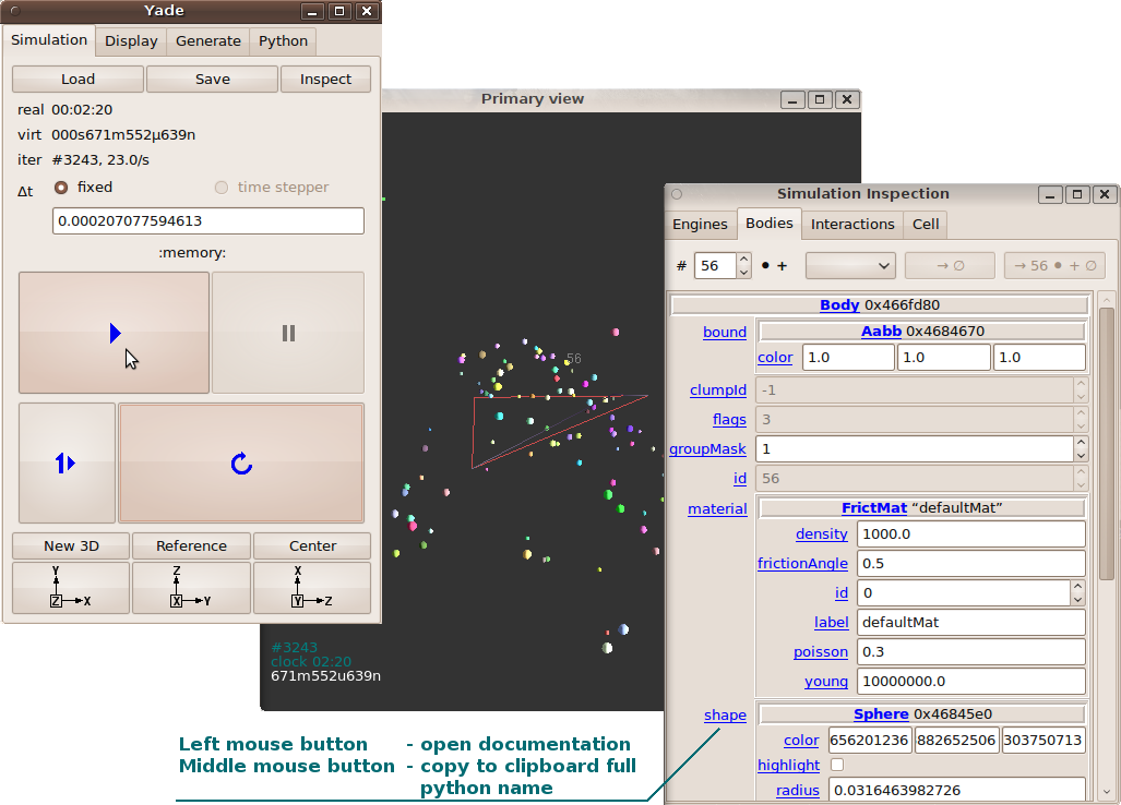
The control window on the left (fig. imgQtGui) is called Controller (can be invoked by yade.qt.Controller() from python or by pressing F12 key in terminal):

The Simulation tab is mostly self-explanatory, and permits basic simulation control.
The Display tab has various rendering-related options, which apply to all opened views (they can be zero or more, new one is opened by the New 3D button).
The Python tab has only a simple text entry area; it can be useful to enter python commands while the command-line is blocked by running script, for instance.

Inside the Inspect window (on the right in fig. imgQtGui) all simulation data can be examined and modified in realtime.

Clicking left mouse button on any of the blue hyperlinks will open documentation.
Clicking middle mouse button will copy the fully qualified python name into clipboard, which can be pasted into terminal by clicking middle mouse button in the terminal (or pressing Ctrl-V).

3d views can be controlled using mouse and keyboard shortcuts; help is displayed if you press the h key while in the 3d view. Note that having the 3d view open can slow down running simulation significantly, it is meant only for quickly checking whether the simulation runs smoothly. Advanced post-processing is described in dedicated section Data mining.

Architecture overview¶

In the following, a high-level overview of Yade architecture will be given. As many of the features are directly represented in simulation scripts, which are written in Python, being familiar with this language will help you follow the examples. For the rest, this knowledge is not strictly necessary and you can ignore code examples.

Data and functions¶

To assure flexibility of software design, yade makes clear distinction of 2 families of classes: data components and functional components. The former only store data without providing functionality, while the latter define functions operating on the data. In programming, this is known as visitor pattern (as functional components “visit” the data, without being bound to them explicitly).

Entire simulation, i.e. both data and functions, are stored in a single Scene object. It is accessible through the Omega class in python (a singleton), which is by default stored in the O global variable:

Yade [28]: O.bodies       # some data components
Out[28]: <yade.wrapper.BodyContainer at 0x7f908ad058c8>

Yade [29]: len(O.bodies)  # there are no bodies as of yet
Out[29]: 0

Yade [30]: O.engines      # functional components, empty at the moment
Out[30]: []

Data components¶

Bodies¶

Yade simulation (class Scene, but hidden inside Omega in Python) is represented by Bodies, their Interactions and resultant generalized forces (all stored internally in special containers).

Each Body comprises the following:

Shape: represents particle’s geometry (neutral with regards to its spatial orientation), such as Sphere, Facet or inifinite Wall; it usually does not change during simulation.
Material: stores characteristics pertaining to mechanical behavior, such as Young’s modulus or density, which are independent on particle’s shape and dimensions; usually constant, might be shared amongst multiple bodies.
State: contains state variables, in particular spatial position and orientation, linear and angular velocity; it is updated by the integrator at every step. The derived classes would contain other information related to current state of this body, e.g. its temperature, averaged damage or broken links between components.
Bound: is used for approximate (“pass 1”) contact detection; updated as necessary following body’s motion. Currently, Aabb is used most often as Bound. Some bodies may have no Bound, in which case they are exempt from contact detection.

(In addition to these 4 components, bodies have several more minor data associated, such as Body::id or Body::mask.)

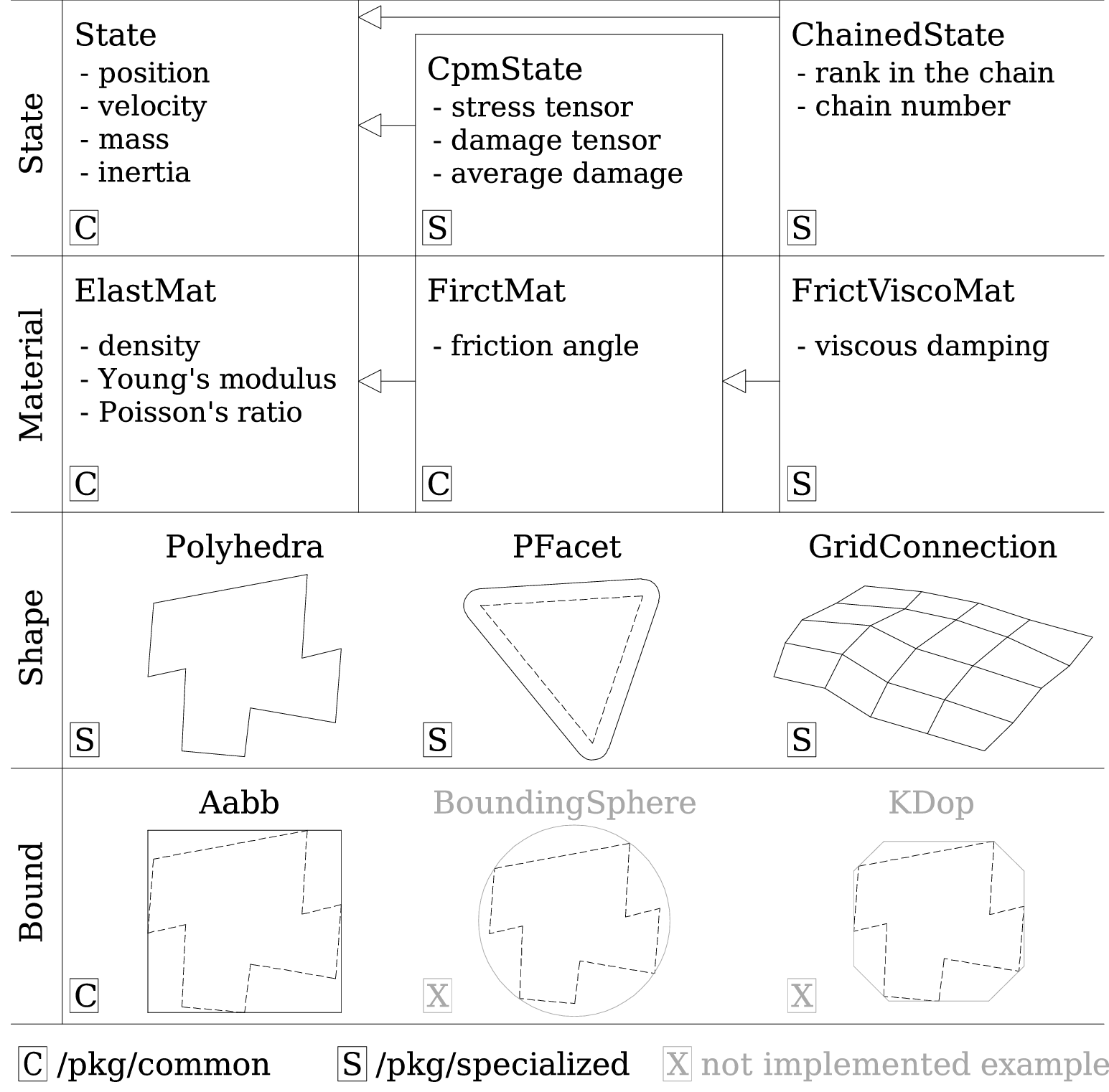
Examples of concrete classes that might be used to describe a Body: State, CpmState, ChainedState, Material, ElastMat, FrictMat, FrictViscoMat, Shape, Polyhedra, PFacet, GridConnection, Bound, Aabb.

All these four properties can be of different types, derived from their respective base types. Yade frequently makes decisions about computation based on those types: Sphere + Sphere collision has to be treated differently than Facet + Sphere collision. Objects making those decisions are called Dispatchers and are essential to understand Yade’s functioning; they are discussed below.

Explicitly assigning all 4 properties to each particle by hand would be not practical; there are utility functions defined to create them with all necessary ingredients. For example, we can create sphere particle using utils.sphere:

Yade [31]: s=utils.sphere(center=[0,0,0],radius=1)

Yade [32]: s.shape, s.state, s.mat, s.bound
Out[32]: 
(<Sphere instance at 0x2de18c0>,
 <State instance at 0xf4ec30>,
 <FrictMat instance at 0x1ac3fb0>,
 None)

Yade [33]: s.state.pos
Out[33]: Vector3(0,0,0)

Yade [34]: s.shape.radius
Out[34]: 1.0

We see that a sphere with material of type FrictMat (default, unless you provide another Material) and bounding volume of type Aabb (axis-aligned bounding box) was created. Its position is at the origin and its radius is 1.0. Finally, this object can be inserted into the simulation; and we can insert yet one sphere as well.

Yade [35]: O.bodies.append(s)
Out[35]: 0

Yade [36]: O.bodies.append(utils.sphere([0,0,2],.5))
Out[36]: 1

In each case, return value is Body.id of the body inserted.

Since till now the simulation was empty, its id is 0 for the first sphere and 1 for the second one. Saving the id value is not necessary, unless you want to access this particular body later; it is remembered internally in Body itself. You can address bodies by their id:

Yade [37]: O.bodies[1].state.pos
Out[37]: Vector3(0,0,2)

Yade [38]: O.bodies[100]    # error because there are only two bodies
---------------------------------------------------------------------------
IndexError                                Traceback (most recent call last)
/builds/yade-dev/trunk/install/lib/x86_64-linux-gnu/yade-ci/py/yade/__init__.py in <module>()
----> 1 O.bodies[100]    # error because there are only two bodies

IndexError: Body id out of range.

Adding the same body twice is, for reasons of the id uniqueness, not allowed:

Yade [39]: O.bodies.append(s)  # error because this sphere was already added
---------------------------------------------------------------------------
IndexError                                Traceback (most recent call last)
/builds/yade-dev/trunk/install/lib/x86_64-linux-gnu/yade-ci/py/yade/__init__.py in <module>()
----> 1 O.bodies.append(s)  # error because this sphere was already added

IndexError: Body already has id 0 set; appending such body (for the second time) is not allowed.

Bodies can be iterated over using standard python iteration syntax:

Yade [40]: for b in O.bodies:
   ....:    print(b.id,b.shape.radius)
   ....: 
0 1.0
1 0.5

Interactions¶

Interactions are always between pair of bodies; usually, they are created by the collider based on spatial proximity; they can, however, be created explicitly and exist independently of distance. Each interaction has 2 components:

IGeom

holding geometrical configuration of the two particles in collision; it is updated automatically as the particles in question move and can be queried for various geometrical characteristics, such as penetration distance or shear strain.

Based on combination of types of Shapes of the particles, there might be different storage requirements; for that reason, a number of derived classes exists, e.g. for representing geometry of contact between Sphere+Sphere, Cylinder+Sphere etc. Note, however, that it is possible to represent many type of contacts with the basic sphere-sphere geometry (for instance in Ig2_Wall_Sphere_ScGeom).

IPhys

representing non-geometrical features of the interaction; some are computed from Materials of the particles in contact using some averaging algorithm (such as contact stiffness from Young’s moduli of particles), others might be internal variables like damage.

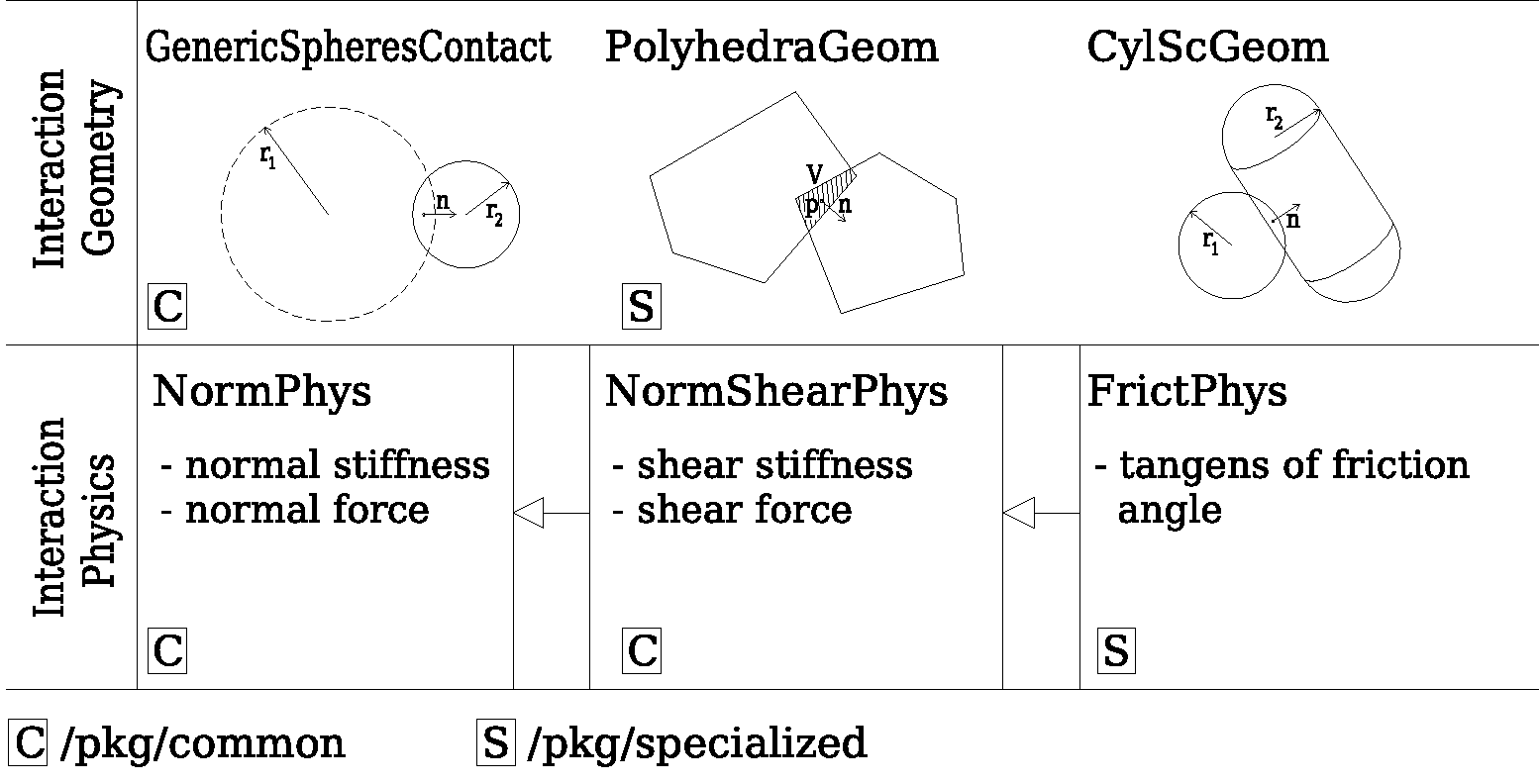
Examples of concrete classes that might be used to describe an Interaction: IGeom, GenericSpheresContact, PolyhedraGeom, CylScGeom, IPhys, NormPhys, NormShearPhys, FrictPhys.

Suppose now interactions have been already created. We can access them by the id pair:

Yade [41]: O.interactions[0,1]
Out[41]: <Interaction instance at 0x2432ab0>

Yade [42]: O.interactions[1,0]     # order of ids is not important
Out[42]: <Interaction instance at 0x2432ab0>

Yade [43]: i=O.interactions[0,1]

Yade [44]: i.id1,i.id2
Out[44]: (0, 1)

Yade [45]: i.geom
Out[45]: <ScGeom instance at 0x236d0a0>

Yade [46]: i.phys
Out[46]: <FrictPhys instance at 0x155e0e0>

Yade [47]: O.interactions[100,10111]     # asking for non existing interaction throws exception
---------------------------------------------------------------------------
IndexError                                Traceback (most recent call last)
/builds/yade-dev/trunk/install/lib/x86_64-linux-gnu/yade-ci/py/yade/__init__.py in <module>()
----> 1 O.interactions[100,10111]     # asking for non existing interaction throws exception

IndexError: No such interaction

Generalized forces¶

Generalized forces include force, torque and forced displacement and rotation; they are stored only temporariliy, during one computation step, and reset to zero afterwards. For reasons of parallel computation, they work as accumulators, i.e. only can be added to, read and reset.

Yade [48]: O.forces.f(0)
Out[48]: Vector3(0,0,0)

Yade [49]: O.forces.addF(0,Vector3(1,2,3))

Yade [50]: O.forces.f(0)
Out[50]: Vector3(1,2,3)

You will only rarely modify forces from Python; it is usually done in c++ code and relevant documentation can be found in the Programmer’s manual.

Function components¶

In a typical DEM simulation, the following sequence is run repeatedly:

reset forces on bodies from previous step
approximate collision detection (pass 1)
detect exact collisions of bodies, update interactions as necessary
solve interactions, applying forces on bodies
apply other external conditions (gravity, for instance).
change position of bodies based on forces, by integrating motion equations.

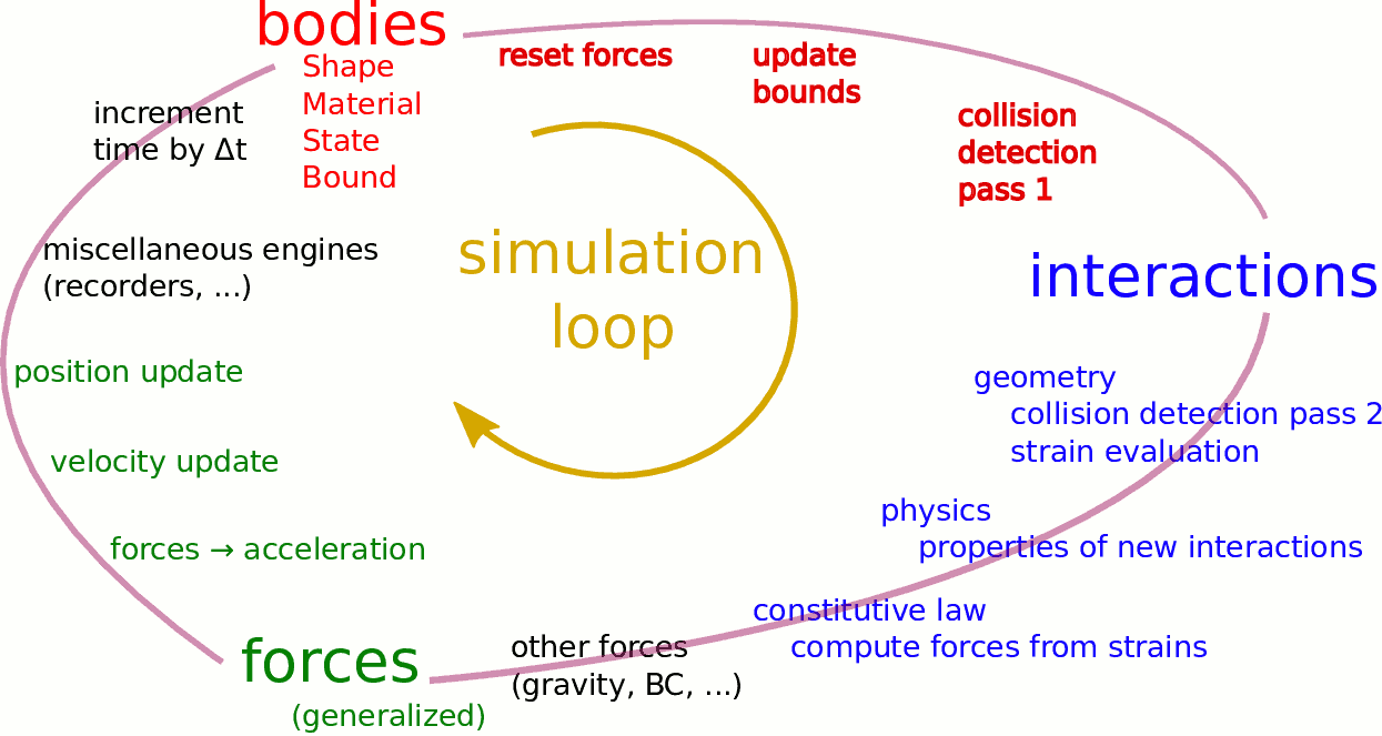
Typical simulation loop; each step begins at body-centered bit at 11 o’clock, continues with interaction bit, force application bit, miscellanea and ends with time update.

Each of these actions is represented by an Engine, functional element of simulation. The sequence of engines is called simulation loop.

Engines¶

Simulation loop, shown at fig. img-yade-iter-loop, can be described as follows in Python (details will be explained later); each of the O.engines items is instance of a type deriving from Engine:

O.engines=[
        # reset forces
        ForceResetter(),
        # approximate collision detection, create interactions
        InsertionSortCollider([Bo1_Sphere_Aabb(),Bo1_Facet_Aabb()]),
        # handle interactions
        InteractionLoop(
                [Ig2_Sphere_Sphere_ScGeom(),Ig2_Facet_Sphere_ScGeom()],
                [Ip2_FrictMat_FrictMat_FrictPhys()],
                [Law2_ScGeom_FrictPhys_CundallStrack()],
        ),
        # apply other conditions
        GravityEngine(gravity=(0,0,-9.81)),
        # update positions using Newton's equations
        NewtonIntegrator()
]

There are 3 fundamental types of Engines:

GlobalEngines: operating on the whole simulation (e.g. ForceResetter which zeroes forces acting on bodies or GravityEngine looping over all bodies and applying force based on their mass)
PartialEngine: operating only on some pre-selected bodies (e.g. ForceEngine applying constant force to some selected bodies)
Dispatchers: do not perform any computation themselves; they merely call other functions, represented by function objects, Functors. Each functor is specialized, able to handle certain object types, and will be dispatched if such obejct is treated by the dispatcher.

Dispatchers and functors¶

For approximate collision detection (pass 1), we want to compute bounds for all bodies in the simulation; suppose we want bound of type axis-aligned bounding box. Since the exact algorithm is different depending on particular shape, we need to provide functors for handling all specific cases. In the O.engines=[…] declared above, the line:

InsertionSortCollider([Bo1_Sphere_Aabb(),Bo1_Facet_Aabb()])

creates InsertionSortCollider (it internally uses BoundDispatcher, but that is a detail). It traverses all bodies and will, based on shape type of each body, dispatch one of the functors to create/update bound for that particular body. In the case shown, it has 2 functors, one handling spheres, another facets.

The name is composed from several parts: Bo (functor creating Bound), which accepts 1 type Sphere and creates an Aabb (axis-aligned bounding box; it is derived from Bound). The Aabb objects are used by InsertionSortCollider itself. All Bo1 functors derive from BoundFunctor.

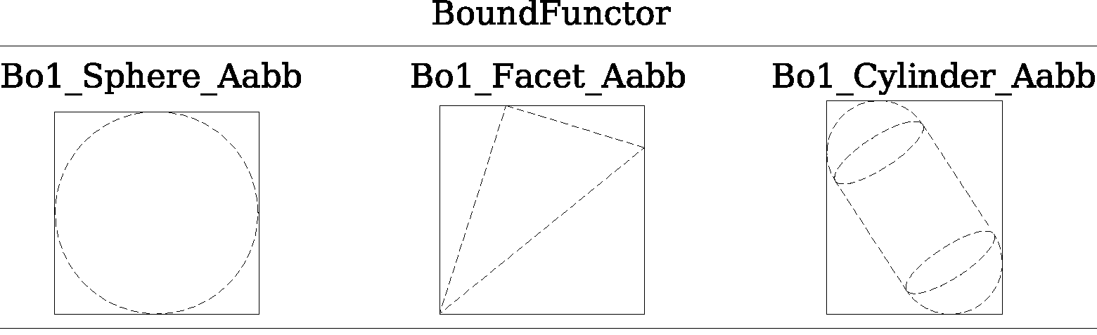
Example bound functors producing Aabb accepting various different types, such as Sphere, Facet or Cylinder. In the case shown, the Bo1 functors produce Aabb instances from single specific Shape, hence the number 1 in the functor name. Each of those functors uses specific geometry of the Shape i.e. position of nodes in Facet or radius of sphere to calculate the Aabb.

The next part, reading

InteractionLoop(
        [Ig2_Sphere_Sphere_ScGeom(),Ig2_Facet_Sphere_ScGeom()],
        [Ip2_FrictMat_FrictMat_FrictPhys()],
        [Law2_ScGeom_FrictPhys_CundallStrack()],
),

hides 3 internal dispatchers within the InteractionLoop engine; they all operate on interactions and are, for performance reasons, put together:

IGeomDispatcher which uses IGeomFunctor

uses the first set of functors (Ig2), which are dispatched based on combination of 2 Shapes objects. Dispatched functor resolves exact collision configuration and creates an Interaction Geometry IGeom (whence Ig in the name) associated with the interaction, if there is collision. The functor might as well determine that there is no real collision even if they did overlap in the approximate collision detection (e.g. the Aabb did overlap, but the shapes did not). In that case the attribute is set to false and interaction is scheduled for removal.

The first functor, Ig2_Sphere_Sphere_ScGeom, is called on interaction of 2 Spheres and creates ScGeom instance, if appropriate.
The second functor, Ig2_Facet_Sphere_ScGeom, is called for interaction of Facet with Sphere and might create (again) a ScGeom instance.

All Ig2 functors derive from IGeomFunctor (they are documented at the same place).

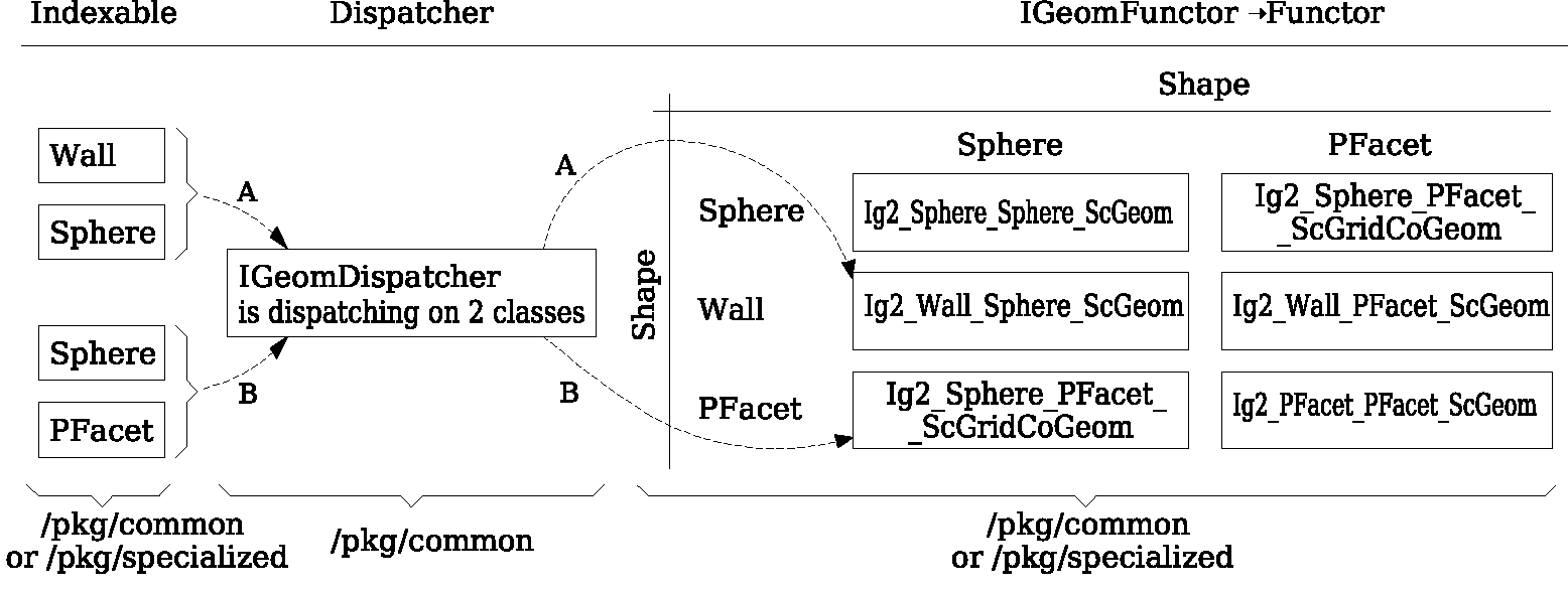
Example interaction geometry functors producing ScGeom or ScGridCoGeom accepting two various different types (hence 2 in their name Ig2), such as Sphere, Wall or PFacet. Each of those functors uses specific geometry of the Shape i.e. position of nodes in PFacet or radius of sphere to calculate the interaction geometry.

IPhysDispatcher which uses IPhysFunctor

dispatches to the second set of functors based on combination of 2 Materials; these functors return return IPhys instance (the Ip prefix). In our case, there is only 1 functor used, Ip2_FrictMat_FrictMat_FrictPhys, which create FrictPhys from 2 FrictMat’s.

Ip2 functors are derived from IPhysFunctor.

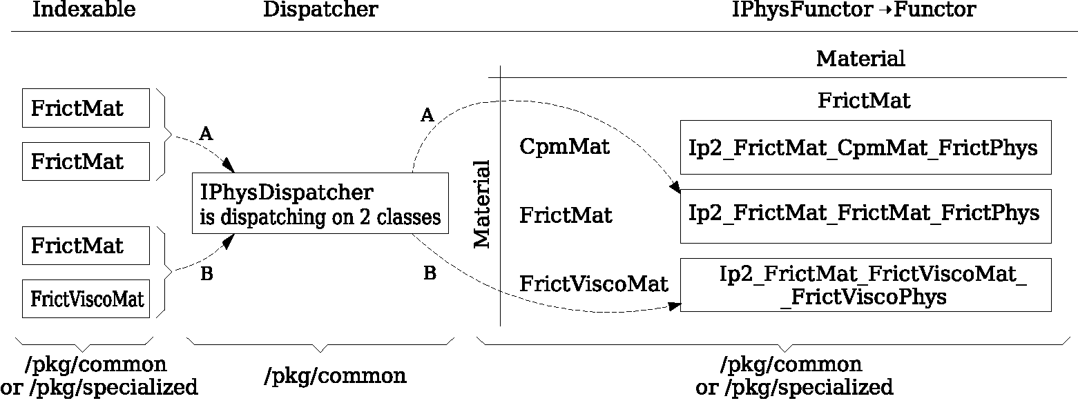
Example interaction physics functors (Ip2_FrictMat_CpmMat_FrictPhys, Ip2_FrictMat_FrictMat_FrictPhys and Ip2_FrictMat_FrictViscoMat_FrictViscoPhys) producing FrictPhys or FrictViscoPhys accepting two various different types of Material (hence Ip2), such as CpmMat, FrictMat or FrictViscoMat.

LawDispatcher which uses LawFunctor

dispatches to the third set of functors, based on combinations of IGeom and IPhys (wherefore 2 in their name again) of each particular interaction, created by preceding functors. The Law2 functors represent constitutive law; they resolve the interaction by computing forces on the interacting bodies (repulsion, attraction, shear forces, …) or otherwise update interaction state variables.

Law2 functors all inherit from LawFunctor.

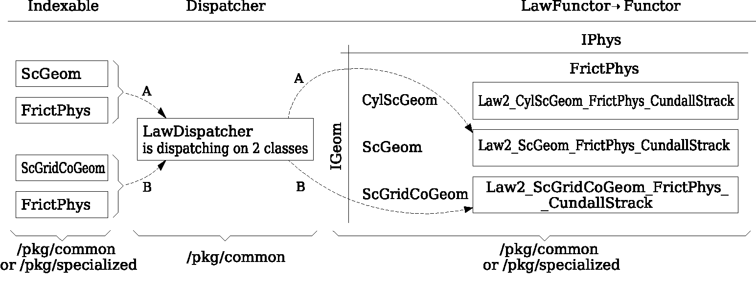
Example LawFunctors (Law2_CylScGeom_FrictPhys_CundallStrack, Law2_ScGeom_FrictPhys_CundallStrack and Law2_ScGridCoGeom_FrictPhys_CundallStrack) each of them performing calcuation of forces according to selected constitutive law.

There is chain of types produced by earlier functors and accepted by later ones; the user is responsible to satisfy type requirement (see img. img-dispatch-loop). An exception (with explanation) is raised in the contrary case.

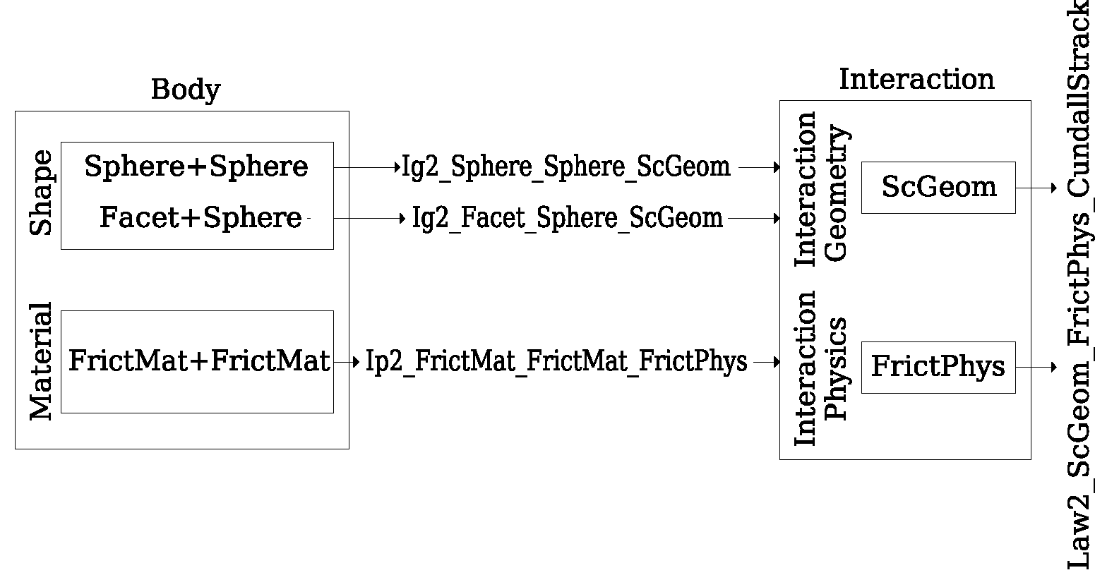
Chain of functors producing and accepting certain types. In the case shown, the Ig2 functors produce ScGeom instances from all handled Shapes combinations; the Ig2 functor produces FrictMat. The constitutive law functor Law2 accepts the combination of types produced. Note that the types are stated in the functor’s class names.

Note

When Yade starts, O.engines is filled with a reasonable default list, so that it is not strictly necessary to redefine it when trying simple things. The default scene will handle spheres, boxes, and facets with frictional properties correctly, and adjusts the timestep dynamically. You can find an example in examples/simple-scene/simple-scene-default-engines.py.