Setting up a simulation¶

Parametric studies¶

Input parameters of the simulation (such as size distribution, damping, various contact parameters, …) influence the results, but frequently an analytical relationship is not known. To study such influence, similar simulations differing only in a few parameters can be run and results compared. Yade can be run in batch mode, where one simulation script is used in conjunction with parameter table, which specifies parameter values for each run of the script. Batch simulation are run non-interactively, i.e. without user intervention; the user must therefore start and stop the simulation explicitly.

Suppose we want to study the influence of damping on the evolution of kinetic energy. The script has to be adapted at several places:

We have to make sure the script reads relevant parameters from the parameter table. This is done using utils.readParamsFromTable; the parameters which are read are created as variables in the yade.params.table module:
```
readParamsFromTable(damping=.2)      # yade.params.table.damping variable will be created
from yade.params import table              # typing table.damping is easier than yade.params.table.damping
```
Note that utils.readParamsFromTable takes default values of its parameters, which are used if the script is not run in non-batch mode.
Parameters from the table are used at appropriate places:
```
NewtonIntegrator(damping=table.damping),
```

The simulation is run non-interactively; we must therefore specify at which point it should stop:

O.engines+=[PyRunner(iterPeriod=1000,command='checkUnbalancedForce()')]    # call our function defined below periodically

def checkUnbalancedForce():
   if unbalancedForce<0.05:                            # exit Yade if unbalanced force drops below 0.05
      plot.saveDataTxt(O.tags['d.id']+'.data.bz2')     # save all data into a unique file before exiting
      import sys
      sys.exit(0)                                      # exit the program

Finally, we must start the simulation at the very end of the script:

O.run()               # run forever, until stopped by checkUnbalancedForce()
waitIfBatch()         # do not finish the script until the simulation ends; does nothing in non-batch mode

The parameter table is a simple text-file (e.g. params.txt ), where each line specifies a simulation to run:

# comments start with # as in python
damping     # first non-comment line is variable name
.2
.4
.6

Finally, the simulation is run using the special batch command:

user@machine:~$ yade-batch params.txt simulation.py

Exercises

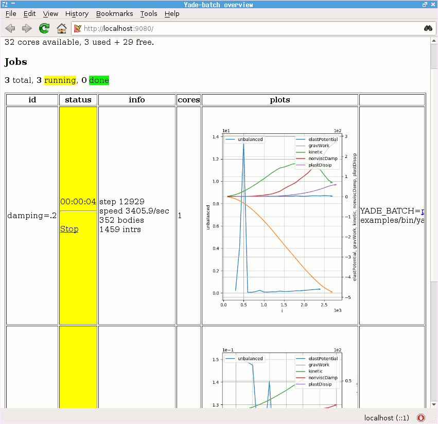
Run the Gravity deposition script in batch mode, varying damping to take values of .2, .4, .6.
See the http://localhost:9080 overview page while the batch is running (fig. imgBatchExample).

Boundary¶

Particles moving in infinite space usually need some constraints to make the simulation meaningful.

Supports¶

So far, supports (unmovable particles) were providing necessary boundary: in the Gravity deposition script the geom.facetBox is internally composed of facets (triangulation elements), which are fixed in space; facets are also used for arbitrary triangulated surfaces (see relevant sections of the User’s manual). Another frequently used boundary is utils.wall (infinite axis-aligned plane).

Periodic¶

Periodic boundary is a “boundary” created by using periodic (rather than infinite) space. Such boundary is activated by O.periodic=True , and the space configuration is decribed by O.cell . It is well suited for studying bulk material behavior, as boundary effects are avoided, leading to smaller number of particles. On the other hand, it might not be suitable for studying localization, as any cell-level effects (such as shear bands) have to satisfy periodicity as well.

The periodic cell is described by its reference size of box aligned with global axes, and current transformation, which can capture stretch, shear and rotation. Deformation is prescribed via velocity gradient, which updates the transformation before the next step. Homothetic deformation can smear velocity gradient accross the cell, making the boundary dissolve in the whole cell.

Stress and strains can be controlled with PeriTriaxController; it is possible to prescribe mixed strain/stress goal state using PeriTriaxController.stressMask.

The following creates periodic cloud of spheres and compresses to achieve \(\sigma_x\)=-10 kPa, \(\sigma_y\)=-10kPa and \(\eps_z\)=-0.1. Since stress is specified for \(y\) and \(z\), stressMask is binary 0b011 (x→1, y→2, z→4, in decimal 1+2=3).

Yade [1]: sp=pack.SpherePack()

Yade [2]: sp.makeCloud((1,1,1),(2,2,2),rMean=.16,periodic=True)
Out[2]: 21

Yade [3]: sp.toSimulation()             # implicitly sets O.periodic=True, and O.cell.refSize to the packing period size
Out[3]: [4, 5, 6, 7, 8, 9, 10, 11, 12, 13, 14, 15, 16, 17, 18, 19, 20, 21, 22, 23, 24]

Yade [4]: O.engines+=[PeriTriaxController(goal=(-1e4,-1e4,-.1),stressMask=0b011,maxUnbalanced=.2,doneHook='functionToRunWhenFinished()')]

When the simulation runs, PeriTriaxController takes over the control and calls doneHook when goal is reached. A full simulation with PeriTriaxController might look like the following:

from yade import pack, plot
sp = pack.SpherePack()
rMean = .05
sp.makeCloud((0, 0, 0), (1, 1, 1), rMean=rMean, periodic=True)
sp.toSimulation()
O.engines = [
        ForceResetter(),
        InsertionSortCollider([Bo1_Sphere_Aabb()], verletDist=.05 * rMean),
        InteractionLoop([Ig2_Sphere_Sphere_ScGeom()], [Ip2_FrictMat_FrictMat_FrictPhys()], [Law2_ScGeom_FrictPhys_CundallStrack()]),
        NewtonIntegrator(damping=.6),
        PeriTriaxController(
                goal=(-1e6, -1e6, -.1), stressMask=0b011, maxUnbalanced=.2, doneHook='goalReached()', label='triax', maxStrainRate=(.1, .1, .1), dynCell=True
        ),
        PyRunner(iterPeriod=100, command='addPlotData()')
]
O.dt = .5 * utils.PWaveTimeStep()
O.trackEnergy = True


def goalReached():
	print('Goal reached, strain', triax.strain, ' stress', triax.stress)
	O.pause()


def addPlotData():
	plot.addData(
	        sx=triax.stress[0],
	        sy=triax.stress[1],
	        sz=triax.stress[2],
	        ex=triax.strain[0],
	        ey=triax.strain[1],
	        ez=triax.strain[2],
	        i=O.iter,
	        unbalanced=utils.unbalancedForce(),
	        totalEnergy=O.energy.total(),
	        **O.energy  # plot all energies
	)


plot.plots = {
        'i': (('unbalanced', 'go'), None, 'kinetic'),
        ' i': ('ex', 'ey', 'ez', None, 'sx', 'sy', 'sz'),
        'i ': (O.energy.keys, None, ('totalEnergy', 'bo'))
}
plot.plot()
O.saveTmp()
O.run()

Setting up a simulation¶

Parametric studies¶

Boundary¶

Supports¶

Periodic¶

Table Of Contents

Previous topic

Next topic

This Page