Potential Particles and Potential Blocks
The origins of scientific development regarding the algorithms described in this section are traced back to: [Boon2012] (Potential Blocks code), [Boon2013b] (Potential Particles code) and [Boon2015] (Block Generation code).
Introduction
This section discusses two codes to simulate (i) non-spherical particles using the concept of the Potential Particles [Houlsby2009], with the solution procedures in [Boon2013] for 3-D and (ii) polyhedral blocks using planar linear inequalities, based on linear programming concepts [Boon2012]. These codes define two shape classes in YADE, namely PotentialParticle and PotentialBlock. Besides some similarities in syntax, they have distinct differences, concerning morphological characteristics of the particles and the methods used to facilitate contact detection.
The Potential Particles code (abbreviated herein as PP) is detailed in [Boon2013], where non-spherical particles are assembled as a combination of 2nd degree polynomial functions and a fraction of a sphere, while their edges are rounded with a user-defined radius of curvature.
The Potential Blocks code (abbreviated herein as PB) is used to simulate polyhedral particles with flat surfaces, based on the work of [Boon2012], where a smooth, inner potential particle is used to calculate the contact normal vector. This code is compatible with the Block Generation algorithm defined in [Boon2015], in which Potential Blocks can be generated by intersections of original, intact blocks with discontinuity planes.
These two codes are independent, in the sense that either one of them can be compiled/used separately, without enabling the other, while they do not interact with each other (i.e. we cannot establish contact between a PP and a PB). Enabling the PB code causes an automatic compilation of the Block Generation algorithm.
Potential Particles code (PP)
The concept of Potential Particles was introduced and developed by [Houlsby2009]. The problem of contact detection between a pair of potential particles was cast as a constrained optimization problem, where the equations are solved using the Newton-Raphson method in 2-D. In [Boon2013] it was extended to 3-D and more robust solutions were proposed. Many numerical optimization solvers generally cannot cope with discontinuities, ill-conditioned gradients (Jacobians) or curvatures (Hessians), and these obstacles were overcome in [Boon2013], by re-formulating the problem and solving the equations using conic optimization solvers. Previous versions made use of MOSEK (using its academic licence), while currently an in-house code written by [Boon2013] is used to solve the conic optimization problem. A potential particle is defined as in (1) [Houlsby2009]:
(1)¶\[\begin{split}f=(1-k) \Bigg(\sum_{i=1}^{N} \langle a_{i}x+b_{i}y+c_{i}z-d_i\rangle ^2-r^2 \Bigg) +k (x^2+y^2+z^2-R^2)\\\end{split}\]
where \((a_i, b_i, c_i)\) is the normal vector of the \(i^{th}\) plane, defined with respect to the particle’s local coordinate system and \(d_i\) is the distance of the plane to the local origin. \(\langle \;\rangle\) are Macaulay brackets, i.e., \(〈x〉 = x\) for \(x > 0\); \(\langle x \rangle = 0\) for \(x \leq 0\). The planes are assembled such that their normal vectors point outwards. They are summed quadratically and expanded by a distance r, which is also related to the radius of the curvature at the corners. Furthermore, a “shadow” spherical particle is added; R is the radius of the sphere, with \(0 < k \; \leq \; 1\), denoting the fraction of sphericity of the particle. The geometry of some cuboidal potential particles is displayed in Fig. fig-pp, for different values of the parameter \(k\).
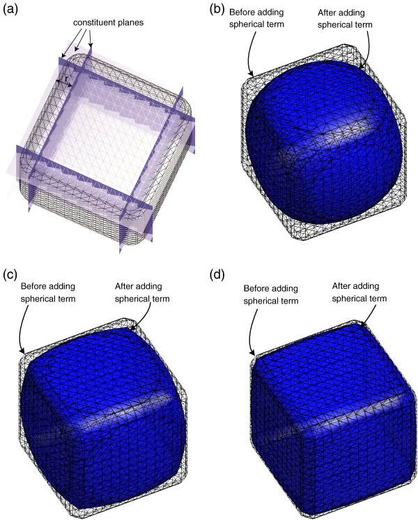
Construction of potential particles (a) constituent planes are squared and expanded by a constant r. A fraction of sphere is added. Particles with the spherical term are visible in (b) k=0.9, (c) k=0.7, and (d) k=0.4 (after [Boon2013]).
The potential function is normalized for computational reasons in the form (2) [Houlsby2009]:
(2)¶\[\begin{split}f=(1-k) \Bigg(\sum_{i=1}^{N} \frac{ \langle a_{i}x+b_{i}y+c_{i}z-d_i\rangle^2 }{ r^2 } -1 \Bigg) +k \Bigg( \frac{ x^2+y^2+z^2 }{ R^2 }-1 \Bigg)\\\end{split}\]
This potential function takes values:
\(f=0\): on the particle surface
\(f<0\): inside the particle
\(f>0\): outside the particle
To ensure numerical stability, it is not advised to use values approaching k=0. In particular, the extreme value k=0 cannot be used from a theoretical standpoint, since the Potential Particles were formulated for strictly convex shapes (curved faces).
Potential Blocks code (PB)
The Potential Blocks code was developed during the D.Phil. thesis of CW Boon [Boon2013b] and discussed in [Boon2012]. It was developed originally for rock engineering applications, to model polygonal and polyhedral blocks with flat surfaces. The blocks are defined with linear inequalities only and unlike the PotentialParticle shape class, no spherical term is considered (so, practically k=0). Although k and R are input parameters of the PotentialBlock shape class, their existence during computation is null. In particular, R is used within the source code, denoting a characteristic dimension of the blocks, but does not reflect the radius of a “shadow particle”, like it does for the Potential Particles. This value of R is used in the Potential Blocks code to calculate the initial bi-section step size for line search, to obtain a point on the particle, which in turn is used to calculate the overlap distance during contact.
For a convex particle defined by N planes, the space that it occupies can be defined using the following inequalities (3):
(3)¶\[\begin{split}a_{i}x + b_{i}y + c_{i}z \; \leq \; d_{i}, i=1:N\\\end{split}\]
where \((a_i, b_i, c_i)\) is the unit normal vector of the \(i^{th}\) plane, defined with respect to the particle’s local coordinate system, and \(d_i\) is the distance of the plane to the local origin. According to [Boon2012], an inner, smooth potential particle is used to calculate the contact normal, formulated as in (4):
(4)¶\[\begin{split}f=\sum_{i=1}^{N} \langle a_{i}x + b_{i}y + c_{i}z - d_i + r\rangle^2\\\end{split}\]
This potential particle is defined inner by a distance r inside the actual particle, with edges rounded by a radius or curvature r, as well (see Fig. fig-pbInner).
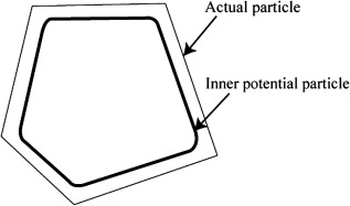
A potential particle is defined inside the actual particle. The normal vector of the particle at any point can be calculated from the first derivative of the potential particle. (after [Boon2012]).
In YADE, the Potential Blocks have a slightly different mathematical expression, since their shape is generated as an assembly of planes as in (5):
(5)¶\[\begin{split}a_{i}x + b_{i}y + c_{i}z - d_{i} - r = 0, i=1:N\\\end{split}\]
while the inner Potential Particle used to calculate the contact normal is defined as in (6):
(6)¶\[\begin{split}f=\sum_{i=1}^{N} \langle a_{i}x + b_{i}y + c_{i}z - d_i\rangle^2.\\\end{split}\]
Now, the Potential Block surface is at a distance of \((d_{i}+r)\) from the local particle center, while the inner potential particle is at a distance \(d\) from the local particle center.
It is worth to emphasize on the fact that the shape of a Potential Block is defined using an assembly of planes and not a single, implicit potential function, like we have for the Potential Particles code. The inner potential particle in the Potential Blocks code is only used to calculate the contact normal.
The problem of establishing intersection between a pair of blocks is cast as a standard linear programming problem of finding a feasible region which satisfies all the linear inequalities defining both blocks. The contact point is calculated as the analytic centre of the feasible region, a well-known concept of interior-point methods in convex optimization calculations. The contact normal is obtained from the gradient of a smooth “potential particle” defined inside the block. The overlap distance is calculated through bi-section searching along the contact normal, within the overlap region.
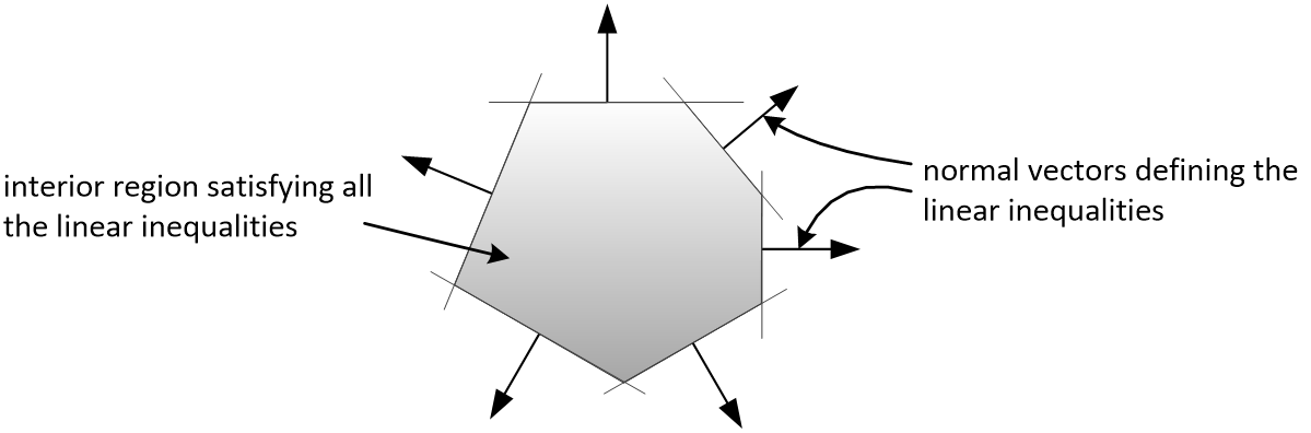
A potential block. The normal vectors of the faces point outwards (after [Boon2013b]).
The linear programming solver for Potential Blocks was originally CPLEX, but has been updated to CLP, developed by COIN-OR, since the latter can be downloaded from Ubuntu or Debian’s distributions without requiring an academic licence.
Engines
The PP and PB codes use their own classes to handle bounding volumes, contact geometry & physics and recording of outputs in vtk format, while they derive the interparticle friction angle from the frictional material class FrictMat. The syntax used to invoke these classes is similar, unless if specified otherwise.
Shape |
||
|---|---|---|
Material |
||
BoundFunctor |
||
IGeom |
||
IGeomFunctor |
||
IPhys |
||
IPhysFunctor |
||
LawFunctor |
||
VTK Recorder |
A simple simulation loop using the Potential Blocks reads as:
O.engines=[
        ForceResetter(),
        InsertionSortCollider([PotentialBlock2AABB()], verletDist=0.01),
        InteractionLoop(
                [Ig2_PB_PB_ScGeom(twoDimension=True, unitWidth2D=1.0, calContactArea=True)],
                [Ip2_FrictMat_FrictMat_KnKsPBPhys(kn_i=1e8, ks_i=1e7, Knormal=1e8, Kshear=1e7, viscousDamping=0.2)],
                [Law2_SCG_KnKsPBPhys_KnKsPBLaw(label='law', neverErase=False, allowViscousAttraction=False)]
        ),
        NewtonIntegrator(damping=0.2, exactAsphericalRot=True, gravity=[0,0,-9.81]),
        PotentialBlockVTKRecorder(fileName='./vtk/file_prefix', iterPeriod=1000, twoDimension=True, sampleX=30, sampleY=30, sampleZ=30, maxDimension=0.2, label='vtkRecorder')
]
Attention should be given to the twoDimension parameter, which defines whether a contact should be handled as 2-D or 3-D.
Contact Law
In both codes, the normal force is calculated as:
(7)¶\[\begin{split}\mathbf{F_{n}}=Knormal \cdot A_{c} \cdot u_{n} \cdot \mathbf{n}\\\end{split}\]
where \(Knormal\) the normal stiffness coefficient \([kN/m^{3}]\); \(A_{c}\) the contact area \([m^{2}]\) and \(u_{n}\) the overlap distance. The normal stiffness of each contact \([kN/m]\) is thus \(k_{n} = Knormal \cdot A_{c}\), where \(A_{c}\) is updated in every timestep.
The shear force is calculated incrementally, using a similar logic. The increment of the shear force vector before slipping of the contact is calculated as:
(8)¶\[\begin{split}\mathbf{\Delta{}F_{s}}=-Kshear \cdot A_{c} \cdot \mathbf{\Delta{}u_{s}}\\\end{split}\]
where \(Kshear\) the shear stiffness coefficient \([kN/m^{3}]\) and \(\Delta{}u_{s}\) the current relative shear displacement.
Contact Area
The contact area is calculated using a heuristic algorithm to detect points on the surface of the overlap volume, searching along the contact shear direction. In essence, it is calculated as the area of a 2D slice of the overlap volume along the shear direction, passing from the contact point. If twoDimension=True, the contactArea parameter is calculated as:
if(twoDimension) { phys->contactArea = phys->jointLength*unitWidth2D;}
The unitWidth2D parameter is defined by the user (usually equal to 1.0), denoting the out-of-plane width in 2-D simulations. The contactArea and jointLength parameters are calculated if calContactArea =True. In the opposite case, they are considered equal to 1.0 and the contact law is degenerated to a linear law with constant stiffness. A minimum value is considered for the contactArea, to represent cases where the overlap volume is practically a point.
Overlap distance
The overlap distance \(u_{n}\) is calculated using a bracketed bisection search algorithm along the contact normal direction, to find two opposite points on the surface of the overlap region, starting from the contact point. It is stored in the parameter penetrationDepth, as the distance between these two opposite points.
Shape definition of a PP and a PB
A strong merit of the Potential Particles and the Potential Blocks codes lies in the fact that the geometric definition of the particle shape and the contact detection problem are resolved using only the equations of the faces of the particles. In this way, using a single data structure, there is no need to store information about the vertices or their connectivity to establish contact, a feature that makes them computationally affordable, while all contacts are handled in the same way (there is no need to distinguish among face-face, face-edge, face-vertex, edge-edge, edge-vertex or vertex-vertex contacts). Due to this, the geometry of a particle is defined in the shape class using the values of the normal vectors of the faces and the distances of the faces from the local origin.
For example, to define a cuboid (6 faces) with rounded edges, an edge length of D, centred to its local centroid and aligned to its principal axes, using the Potential Particles code, we set:
r=D/10.
k=0.3
R=D/2.
b=Body()
b.shape=PotentialParticle( r=r, k=k, R=R,
                           a=[   1.0,    -1.0,     0.0,     0.0,     0.0,     0.0],
                           b=[   0.0,     0.0,     1.0,    -1.0,     0.0,     0.0],
                           c=[   0.0,     0.0,     0.0,     0.0,     1.0,    -1.0],
                           d=[D/2.-r,  D/2.-r,  D/2.-r,  D/2.-r,  D/2.-r,  D/2.-r], ...)
The first element of the vector parameters \(a, b, c, d\) refers to the normal vector of the first plane and its distance from the local origin, the second element to the second plane, and so on.
Using the Potential Particles code, this is not a perfect cube, since the particle geometry is defined by a potential function as in (2). It is reminded that within this potential function, these planes are summed quadratically, the particle edges are rounded by a radius of curvature r and then the particle faces are curved by the addition of a “shadow” spherical particle with a radius R, to a percentage defined by the parameter k. A value r is deducted from each element of the vector parameter d, to compensate for expanding the potential particle by r.
The parameters \(a_{i}, b_{i}, c_{i}, d_{i}\) stated above correspond to the planes used in (5):
\[\begin{split}1.0 x + 0.0 y + 0.0 z = D/2 \Leftrightarrow +x=D/2\\ -1.0 x + 0.0 y + 0.0 z = D/2 \Leftrightarrow -x=D/2\\ 0.0 x + 1.0 y + 0.0 z = D/2 \Leftrightarrow +y=D/2\\ 0.0 x - 1.0 y + 0.0 z = D/2 \Leftrightarrow -y=D/2\\ 0.0 x + 0.0 y + 1.0 z = D/2 \Leftrightarrow +z=D/2\\ 0.0 x + 0.0 y - 1.0 z = D/2 \Leftrightarrow -z=D/2\\\end{split}\]
To model a cube with an edge of D, using the Potential Blocks code, we define:
r=D/10.
R=D/2.*sqrt(3)
b=Body()
b.shape=PotentialBlock( r=r, R=R,
                        a=[   1.0,    -1.0,     0.0,     0.0,     0.0,     0.0],
                        b=[   0.0,     0.0,     1.0,    -1.0,     0.0,     0.0],
                        c=[   0.0,     0.0,     0.0,     0.0,     1.0,    -1.0],
                        d=[D/2.-r,  D/2.-r,  D/2.-r,  D/2.-r,  D/2.-r,  D/2.-r], ...)
Using the Potential Blocks code, this particle will have sharp edges and flat faces in what regards its geometry (i.e. the space it occupies), defined by the given planes, while for the calculation of the contact normal, an inner potential particle with rounded edges is used, formulated as in (6), located fully inside the actual particle. The distances of the planes from the local origin, stored in the vector parameter d, are reduced by r to achieve an exact edge length of D, using (5). The value of r must be sufficiently small, so that \(d_{min}-r>0\), while it should be sufficiently large, to allow for a proper calculation of the gradient of the inner Potential Particle at the contact point. A recommended value is \(r \approx 0.5*d_{min}\).
To ensure numerical stability, it is advised to normalize the normal vector of each plane, so that \({a_{i}}^2 + {b_{i}}^2 + {c_{i}}^2 = 1\). There is no limit to the number of the particle faces that can be used, a feature that allows the modelling of a variety of convex particle shapes.
In practice, it is usual for the geometry of a particle to be given in terms of vertices & their connectivity (e.g. in the form of a surface mesh, like in .stl files). In such cases, the user can calculate the normal vector of each face, which will give the coefficients \(a_{i}, b_{i}, c_{i}\) and using a vertex of each face, then calculate the coefficients \(d_{i}\). A python routine to perform this without any additional effort by the user is currently being developed.
Body definition of a PP and a PB
To define a body using the PotentialParticle or PotentialBlock shape classes, it has to be assembled using the _commonBodySetup function, which can be found in the file py/utils.py. For example, to define a PotentialParticle:
O.materials.append(FrictMat(young=-1,poisson=-1,frictionAngle=radians(0.0),density=2650,label='frictionless'))

b=Body()
b.shape=PotentialParticle(...)
b.aspherical=True # To be used in conjunction with exactAsphericalRot=True in the NewtonIntegrator
# V: Volume
# I11, I22, I33: Principal inertias
utils._commonBodySetup(b,V,Vector3(I11,I22,I33), material='frictionless', pos=(0,0,0), fixed=False)
b.state.pos=Vector3(xPos,yPos,zPos)
b.state.ori=Quaternion((random.random(),random.random(),random.random()),random.random())
b.shape.volume=V;
O.bodies.append(b)
The PotentialParticle must be initially defined, so that the local axes coincide with its principal axes, for which the inertia tensor is diagonal. More specifically, the plane coefficients \((a_i, b_i, c_i)\) defining the plane normals must be rotated, so that when the orientation of the particle is zero, the PotentialParticle is oriented to its principal axes.
It should be noted that the principal inertia values I11, I22, I33 mentioned here are divided with the density of the considered material, since they are multiplied with the density inside the _commonBodySetup function. The mass of the particle is calculated within the same function as well, so we do not need to set manually b.mass=V*density.
For the Potential Particles, the volume and inertia must be calculated manually and assigned to the body as demonstrated above. For the Potential Blocks, an automatic calculation has been implemented for the volume and inertia tensor, the user does not have to define the particle to its principal axes, since this is handled automatically within the source code, while if no value is given for the parameter R, it is calculated as half the distance of the farthest vertices.
For example, to define a PotentialBlock:
O.materials.append(FrictMat(young=-1,poisson=-1,frictionAngle=radians(0.0),density=2650,label='frictionless'))

b=Body()
b.shape=PotentialBlock(R=0.0, ...) #here we set R=0.0 to trigger automatic calculation of R
b.aspherical=True # To be used in conjunction with exactAsphericalRot=True
utils._commonBodySetup(b,b.shape.volume,b.shape.inertia, material='frictionless', pos=Vector3(xPos,yPos,zPos), fixed=False)
b.state.ori=b.shape.orientation # this will rotate the particle to its initial random system. If b.state.ori=Quaternion.Identity, the PB is oriented to its principal axes
O.bodies.append(b)
Boundary Particles
The PP & PB codes support the definition of boundary particles, which interact only with non-boundary ones. These particles can have a variety of uses, e.g. to model loading plates acting on a granular sample, while different uses can emerge for different applications. A particle can be set as a boundary one in both codes, using the boolean parameter isBoundary inside the shape class.
In the PP code, all particles interact with the same normal and shear contact stiffness Knormal and Kshear, defined in the Ip2_FrictMat_FrictMat_KnKsPhys functor.
The PB code supports the definition of different contact stiffness values for interactions between boundary and non-boundary or non-boundary and non-boundary particles.
When isBoundary=False, the PotentialBlock in question is handled to interact with normal and shear stiffness coefficients Knormal and Kshear, respectively, with other non-boundary particles.
When isBoundary=True, the PotentialBlock in question is handled to interact with normal and shear stiffness coefficients kn_i and ks_i, respectively, with non-boundary particles.
Visualization
Visualization of the PotentialParticle and PotentialBlock shape classes is offered using the qt environment (OpenGL). Additionally, the export.VTKExporter.exportPotentialBlocks function and PotentialParticleVTKRecorder and PotentialBlockVTKRecorder engines can be used to export geometrical and interaction information of the analyses in vtk format (visualized in Paraview). It should be noted that currently the PotentialBlockVTKRecorder records a rounded approximation of the particle, rather than the actual particle with sharp corners and edges.
In the qt environment, the PotentialParticle shape class is visualized using the Marching Cubes algorithm, and the level of display accuracy can be determined by the user. This is controlled by the parameters:
# Potential Particles
Gl1_PotentialParticle.sizeX=20
Gl1_PotentialParticle.sizeY=20
Gl1_PotentialParticle.sizeZ=20
A similar choice exists for output in vtk format, using the PotentialParticleVTKRecorder or PotentialBlockVTKRecorder, syntaxed as:
# Potential Particles
PotentialParticleVTKRecorder(sampleX=30, sampleY=30, sampleZ=30, maxDimension=20)

# Potential Blocks
PotentialBlockVTKRecorder(sampleX=30, sampleY=30, sampleZ=30, maxDimension=20)
The parameters sizeX,Y,Z (for OpenGL visualization) and sampleX,Y,Z (for output in vtk format) represent the number of subdivisions of the Aabb of the particle to a grid, which will be used to draw its geometry, in respect to the global axes X, Y, Z. Larger values will result to a more accurate display of the particles’ shape, but will slow down the visualization speed in qt and writing speed of the .vtk files and increase the size of the .vtk files. For output in vtk format, users can also define the parameter maxDimension, which overrides the selected sampleX,Y,Z values if they are too small, as described below:
The PotentialParticleVTKRecorder and PotentialBlockVTKRecorder also support optionally the recording of the particles’ velocities (linear and angular), interaction information (contact point and forces), colors and ids, using:
# Potential Particles
PotentialParticleVTKRecorder(..., REC_VELOCITY=True, REC_INTERACTION=True, REC_COLORS=True, REC_ID=True)

# Potential Blocks
PotentialBlockVTKRecorder(..., REC_VELOCITY=True, REC_INTERACTION=True, REC_COLORS=True, REC_ID=True)
Force chains and other visual outputs are available in qt by default, while they can be extracted in vtk format using the classic VTKRecorder or the export.VTKExporter class.
A boolean parameter twoDimension exists to specify whether the particles will be rendered as 2-D or 3-D in the vtk output:
# Potential Particles
PotentialParticleVTKRecorder(..., twoDimension=False)

# Potential Blocks
PotentialBlockVTKRecorder(..., twoDimension=False)
This parameter should not be mixed up with the Ip2_FrictMat_FrictMat_KnKsPBPhys.twoDimension parameter, which is used to define how the contact forces are calculated, as described in the Engines section.
Axis-Aligned Bounding Box
The PP & PB codes use their own BoundFunctors, called PotentialParticle2AABB and PotentialBlock2AABB, respectively, to define the Axis-Aligned Bounding Box of each particle. In both bound functors, a boolean parameter AabbMinMax exists, allowing the user to choose between an approximate cubic Aabb or a more accurate one.
In particular, if AabbMinMax=False, a cubic Aabb is considered with dimensions 1.0*R. This is implemented for both the PP and PB codes, even though the Potential Blocks do not have a spherical term. In this case, the radius R is used as a reference length, denoting half the diagonal of the cubic Aabb. Usage of this approximate cubic Aabb is not advised in general, since it can increase the number of empty contacts, adding thus to the time needed to facilitate the approximate contact detection, while it relies on the radius R, the value of which should enclose the whole particle if this option is activated.
If AabbMinMax=True, a more accurate Aabb can be defined. Currently, the initial Aabb of a PotentialParticle has to be defined manually by the user, in the particle local coordinate system and for the initial orientation of the particle. To do so, the user has to manually specify the two extreme points of the Aabb: minAabbRotated, maxAabbRotated inside the shape class.
The Aabb for a PotentialBlock, on the other hand, is calculated and updated automatically from the vertices of the particle, if the boolean parameter AabbMinMax =True.
As discussed in the subsection Visualization, the dimensions of the Aabb are used as a drawing space in the code implementing rendering of the particles in the qt environment (for the PP code) and for the creation of the output files in vtk format (for both codes). This is achieved by using two auxiliary parameters: minAabb and maxAabb. For the Potential Blocks code only, if these parameters are left unassigned, the drawing space is configured automatically inside the PotentialBlockVTKRecorder using the Aabb of the particle. For the particles to be properly rendered as closed surfaces in both qt and vtk outputs using the available codes, we need to define a drawing space slightly larger than the actual one. Here, this drawing space is represented by the Aabb of the particles, and thus the differentiation between the minAabb, maxAabb and minAabbRotated, maxAabbRotated stems from the need to satisfy two conditions: 1. The Aabb used for primary contact detection must be as tight as possible, in order to have the least number of empty contacts and 2. The Aabb used as a rendering space must be slightly larger, in order to have proper rendering. If a dimension of the Aabb used for visualization purposes is defined smaller than the actual one, the faces on that side of the particle are rendered as hollow and only the edges are visualised, a functionality that can be used to e.g. see through boundaries, like demonstrated in the vtk output of the examples/PotentialParticles/cubePPscaled.py example.
To recap, in the Potential Particles code, the minAabbRotated and maxAabbRotated parameters define the initial Aabb used to facilitate primary contact detection, while the minAabb and maxAabb parameters are used for visualization of the particles in qt and vtk outputs. In the Potential Blocks code, the Aabb used to facilitate primary contact detection is calculated automatically from the particles’ vertices, which are also used for visualization in qt, while the parameters minAabb and maxAabb are used for visualization in vtk outputs and can be left unassigned, to trigger an automatic configuration of the drawing space of the particle in the PotentialBlockVTKRecorder.
Two brief examples demonstrating the syntax of these features can be found below.
For the Potential Particles code:
b=Body()
b.shape=PotentialParticle(AabbMinMax=True,
                          minAabbRotated=Vector3(xmin,ymin,zmin),
                          maxAabbRotated=Vector3(xmax,ymax,zmax),
                          minAabb=Vector3(xmin,ymin,zmin),
                          maxAabb=Vector3(xmax,ymax,zmax), ...)
For the Potential Blocks code:
b=Body()
b.shape=PotentialBlock(AabbMinMax=True,
                       minAabb=Vector3(xmin,ymin,zmin),
                       maxAabb=Vector3(xmax,ymax,zmax), ...)
Block Generation algorithm
The Potential Blocks code is compatible with the Block Generation algorithm introduced in [Boon2015], which can split particles by their intersection with discontinuity planes, initially developed for the study of rock-masses. This code is hardcoded in YADE in the form of a Preprocessor. Using a single data structure for the definition of the particle shape and the definition of the discontinuities, as well, allows the generation of a large number of particles at a reasonable computational cost. The sequential subdivision concept is used along with a linear programming framework. Non-persistent joints can be modelled by introducing more constraints.
An example to demonstrate the usage of this code exists in examples/PotentialBlocks/WedgeYADE.py The discontinuity planes used in this script are included in a csv format in examples/PotentialBlocks/joints/jointC.csv.
The documentation on how to use this code is currently being written.
Examples
Examples can be found in the folders examples/PotentialParticles and examples/PotentialBlocks/, where the syntax of the codes is demonstrated.
Disclaimer
These codes were developed for academic purposes. Some variables are no longer in use, as the PhD thesis of the original developer spanned over many years, with numerous trials and errors. As this piece of code has many dependencies within the YADE ecosystem, user discretion is advised.
References
To acknowledge our scientific contribution, please cite the following:
\(\underline{\textrm{Potential Blocks}}\)
Boon CW (2013) Distinct Element Modelling of Jointed Rock Masses: Algorithms and Their Verification. D.Phil. Thesis, University of Oxford
Boon CW, Houlsby GT, Utili S (2012) A new algorithm for contact detection between convex polygonal and polyhedral particles in the discrete element method. Computers and Geotechnics, 44: 73-82
\(\underline{\textrm{Potential Particles}}\)
Houlsby GT (2009) Potential particles: a method for modelling non-circular particles in DEM. Computers and Geotechnics, 36(6):953-959
Boon CW, Houlsby GT, Utili S (2013) A new contact detection algorithm for three dimensional non-spherical particles. Powder Technology, S.I. on DEM, 248: 94-102
\(\underline{\textrm{Block Generation}}\)
Boon CW, Houlsby GT, Utili S (2015) A new rock slicing method based on linear programming. Computers and Geotechnics, 65:12-29