Using YADE 1D vertical VANS fluid resolution

The goal of the present note is to detail how the DEM-fluid coupling can be used in practice in YADE. It is complementary with the three notes [Maurin2018_VANSbasis], [Maurin2018_VANSfluidResol] and [Maurin2018_VANSvalidations] detailing respectively the theoretical basis of the fluid momentum balance equation, the numerical resolution, and the validation of the code.

All the coupling and the fluid resolution relies only on the engine HydroForceEngine, which use is detailed here. Examples scripts using HydroForceEngine for different purposes can be found in YADE source code in the folder trunk/examples/HydroForceEngine/. In order to get familiar with this engine, it is recommended to read the present note and test/modify the examples scripts.

DEM-fluid coupling and fluid resolution in YADE

In YADE, the fluid coupling with the DEM is done through the engine called HydroForceEngine, which is coded in the source in the files trunk/pkg/common/HydroForceEngine.cpp and hpp. HydroForceEngine has three main functions:

• It applies drag and buoyancy to each particle from a 1D vertical fluid velocity profile (HydroForceEngine::action)

• It can evaluates the average drag force, particle velocity and solid volume fraction profiles (HydroForceEngine::averageProfile)

• It can solves the fluid velocity equation detailed in the first section, from given average drag force, particle velocity and solid volume fraction profiles (HydroForceEngine::fluidResolution)

We clearly see the link between the three functions. The idea is to evaluate the average profiles from the DEM, put it as input to the fluid resolution, and apply the fluid forces corresponding to the obtained fluid velocity profile to the particles. In the following, the three points will be detailed separately with precision and imaging with the example scripts available in yade source code at trunk/examples/HydroForceEngine/.

Application of drag and buoyancy forces (HydroForceEngine::action)

By default, when adding HydroForceEngine to the list of engine, it applies drag and buoyancy to all the particles which IDs have been passed in argument to HydroForceEngine through the ids variable. This is done for example, in the example script trunk/examples/HydroForceEngine/, in the engine lists:

O.engines = [
ForceResetter(),
...
HydroForceEngine(densFluid = densFluidPY,...,ids = idApplyForce),
...
NewtonIntegrator(gravity=gravityVector, label='newtonIntegr')
]

where \(idApplyForce\) corresponds to a list of particle ID to which the hydrodynamic forces should be applied. The expression of the buoyancy and drag force applied to the particles contained in the id list is detailed below.

In case where the fluid is at rest (HydroForceEngine.steadyFlow = False), HydroForceEngine applies buoyancy on a particle \(p\) from the fluid density and the acceleration of gravity \(g\) as:

\[\mathbf f_b^p = - \rho^f V^p \mathbf g.\]

Meanwhile, if the fluid flow is steady and turbulent, the buoyancy which is related to the fluid pressure gradient does not have a term in the streamwise direction (see discussion p. 5 of [Maurin2018]). Puting the option HydroForceEngine.steadyFlow to True turns the expression of the buoyancy into:

\[\mathbf f_b^p = - \rho^f V^p (\mathbf g.\mathbf e_x) \mathbf e_x.\]

Also, HydroForceEngine applies a drag force to each particles contained in the ids list. This drag force depends on the velocity of the particles and on the fluid velocity, which is defined by a 1D fluid velocity profile, HydroForceEngine.vxFluid. This fluid velocity profile can be evaluated from the fluid model, but can also be imposed by the user and stay constant. From this 1D vertical fluid velocity profile, the drag force applied to particle p reads:

\[\mathbf f_D^p= \frac{1}{2} C_d A \rho^f ||u^f_p \mathbf e_x- \mathbf v^p|| \left(u^f_p \mathbf e_x - \mathbf v^p\right),\]

where \(\mathbf u^f_p\) is the fluid velocity at the center of particle \(p\), \(\mathbf v^p\) is the particle velocity, \(\rho^f\) is the fluid density, \(A = \pi d^2/4\) is the area of the sphere submitted to the flow, and \(C_d\) is the drag coefficient accounts for the effects of particle Reynolds number [Dallavalle1948] and of increased drag due to the presence of other particles (hindrance, [Richardson1954]:

\[C_d = \left(0.44 + \frac{24}{Re_p}\right) (1-\phi_p)^{- \gamma} = \left(0.44 + 24 \frac{\nu^f}{||u^f_p \mathbf e_x- \mathbf v^p|| d}\right) (1-\phi_p)^{- \gamma}\]

with \(\phi_p\) the solid volume fraction at the center of the particle evaluated from HydroForceEngine.phiPart, and \(\gamma\) the Richardson-Zaki exponent, which can be set through the parameter HydroForceEngine.expoRZ (3.1 by default).

HydroForceEngine can also apply a lift force, but this is not done by default (HydroForceEngine.lift = False), and this is not recommended by the author considering the uncertainty on the actual formulation (see discussion p. 6 of [Maurin2015] and [Schmeeckle2007]).

As the fluid velocity profile (HydroForceEngine.vxFluid) and solid volume fraction profile (HydroForceEngine.phiPart) can be imposed by the user, the application of drag and buoyancy to the particles through HydroForceEngine can be done without using the function averageProfile and the fluid resolution. Examples of such use can be found in the source code: trunk/examples/HydroForceEngine/oneWayCouplingfootnote{In this case, we talk about a one-way coupling as the fluid influence the particles but is not influenced back}.

Solid phase averaging (HydroForceEngine::averageProfile)

In order to solve the fluid equation, we have seen that it is necessary to compute from the DEM the solid volume fraction, the solid velocity, and the averaged drag profiles. The function HydroForceEngine.averageProfile() has been set up in order to do so. It is designed to evaluate the average profiles over a regular grid, at the position between two mesh nodes. In order to match the fluid velocity profile numerotation, the averaged vector are of size \(ndimz+1\) even though the quantities at the top and bottom boundaries are not evaluated and set to zero by defaultfootnote{It is not necessary to evaluate the solid DEM quantities at the boundaries are they are not considered in the fluid resolution, see subsection boundaries of [Maurin2018_VANSfluidResol]}. textcolor{red}{You should do that}

The solid volume fraction profile is evaluated by considering the volume of particles contained in the layer considered. The layer is defined by the mesh step along the wall-normal direction, but extend over the whole length and width of the sample. We perform such an averaging only discretized over the wall-normal direction in order to match the fluid resolution. Meanwhile, this is also physical as, at steady state the problem is unidirectional on average, so that the only variation we should observe in the measured averaged quantities should be along the vertical direction, z. Therefore, the solid volume fraction is evaluated by considering the volume of particles which is contained inside the layer considered \(i+1/2\):

\[\phi_{i+1/2} = \sum_{p \in [idz;(i+1)dz]} V^p_{i+1/2};\]

where the sum is over the particles \(p\) which have at least a part of their volume inside the layer \(i+1/2\), i.e. in between an elevation of \(i*dz\) and \((i+1)*dz\), and \(V^p_{i+1/2}\) is the volume of the particles considered which is contained inside the layer considered. The latter correspond to the integral between two points of a slice of sphere and can be evaluated analytically in cylindrical coordinate. Following this formulation and the formalism of [Jackson2000] with a weighting step function, any particle-associated quantity \(K\) can be averaged with the following formulation:

\[\left. \left<K\right>^p \right\rvert_{i+1/2} = \frac{\sum_{p \in [idz;(i+1)dz]} V^p_{i+1/2} K^p}{\sum_{p \in [idz;(i+1)dz]} V^p_{i+1/2}},\]

Where \(K^p\) is the quantity associated with particle \(p\), e.g. the particle streamwise velocity. In this case, we can write:

\[\left<v_x\right>^p\rvert_{i+1/2} = \frac{\sum_{p \in [idz;(i+1)dz]} V^p_{i+1/2} v_x^p}{\sum_{p \in [idz;(i+1)dz]} V^p_{i+1/2}},\]

where \(v_x^p\) is the velocity of particle \(p\). Regarding the evaluation of the average streamwise drag force transmitted by the fluid to the particles, it can be written similarly as:

\[\left<f_{D,x}\right>^p\rvert_{i+1/2} = \frac{\sum_{p \in [idz;(i+1)dz]} V^p_{i+1/2} f^p_{D,x}}{\sum_{p \in [idz;(i+1)dz]} V^p_{i+1/2}},\]

where \(f^p_{D,x}\) is the drag force on particle \(p\).

As will be detailed in the next part, these averaged profile can be used for the fluid resolution, but they can also be used for analysis as done for example for bedload transport in [Maurin2015b] [Maurin2018].

Fluid resolution\HydroForceEngine::fluidResolution

In order to use the fluid resolution inside the fluid-DEM coupling framework, it is necessary to call the function HydroForceEngine.averageProfile() in order to evaluate the averaged solid volume fraction profile, streamwise velocity and streamwise drag force. The latter is necessary in order to evaluate the terms \(\beta\) taken into account in the fluid equation (see [Maurin2018_VANSfluidResol] for details). \(\beta\) is defined as:

\[\left. n\left< f^f_x\right>^p\right\rvert_{i+1/2} = \beta_{i+1/2} \left(\left. \left<u_x\right>^f\right\rvert_{i+1/2} - \left. \left< v_x\right>^p\right\rvert_{i+1/2}\right)\]

so that it can be evaluated directly from the averaged drag, particle velocity and the fluid velocity at the last iteration (explicited the term \(\beta\) in the fluid resolution):

\[\beta_{i+1/2}^n = \frac{\left. n\left< f^f_x\right>^p\right\rvert_{i+1/2}^{n-1} }{\left. \left<u_x\right>^f\right\rvert_{i+1/2}^{n-1} - \left. \left< v_x\right>^p\right\rvert_{i+1/2}^{n-1}}\]

where the solid variables have been denoted with a superscript \(n-1\) as they are known and not re-evaluated at each time stepfootnote{In a way \(\beta^n\) should probably be better written as \(\beta^{n-1}\)}. This terms is called taufsi and is directly evaluated inside the code.

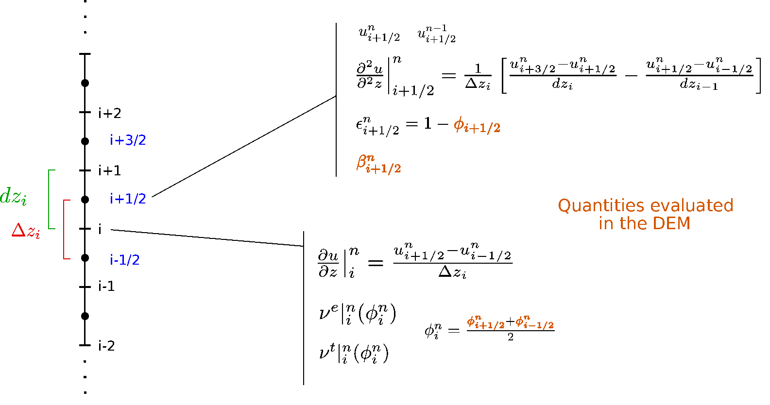
Schematical picture of the numerical fluid resolution and variables definition with a regular mesh. All the definitions still holds for a mesh with variable spatial step.

All the quantities needed in order to solve the fluid resolution - highlighted in [Maurin2018_VANSfluidResol] and recalled in figure fig-scheme - are now explicited. They can be directly evaluated in YADE with the function HydroForceEngine.averageProfile(). From there, the fluid resolution can be performed over a given time \(t_{resol}\) with a given time step \(\Delta t\) by calling directly the function HydroForceEngine.fluidResolution (\(t _{resol}\),\(\Delta t\)). This will perform the fluid resolution described in [Maurin2018_VANSfluidResol], \(N = t_{resol}/\Delta t\) times, with a time step \(\Delta t\), considering the vertical profiles of \(\beta\), \(\left<v_x\right>\) and \(\phi\) as constant in time. Therefore, one should not only be carefull about the time step, but also about the period of coupling, which should not be too large in order to avoid unphysical behavior in the DEM due to a drastic change of velocity profile not compensated by an increased transmitted drag force.

In the example script in YADE source code, trunk/examples/HydroForceEngine/twoWayCoupling/sedimentTransportExample_1DRANSCoupling.py, the DEM and fluid resolution are coupled with a period of \(fluidResolPeriod = 10^{-2}s\) by default, and with a fluid time step of \(dtFluid = 10^{-5}s\). This means that the DEM is let evolved for \(10^{-2}s\), and frozen during the fluid resolution which is made over \(fluidResolPeriod/dtFluid = 10^3\) step with \(\Delta t = 10^{-5}\). Then, the DEM is let evolved again but with a new fluid velocity profile for \(10^{-2}s\), and frozen…etc. This period between two fluid resolution should be tested and taken not too long (see appendix of [Maurin2015b]).

Meanwhile, the fluid resolution can be used in itself, without DEM coupling, in particular to verify the fluid resolution in known cases. This is done in the example folder of YADE source code, trunk/examples/HydroForceEngine/fluidValidation/, where the cases of a poiseuille flow and a log layer have been considered and validated.