Simulating Acoustic Emissions in Yade
Suggested citations:
Summary
This document briefly describes the simulation of acoustic emissions (AE) in Yade. Yade’s clustered strain energy based AE model follows the methods introduced by [Hazzard2000] and [Hazzard2013]. A validation of Yade’s method and a look at the effect of rock heterogeneity on AE during tensile rock failure is discussed in detail in [Caulk2018] and [Caulk2020].
Model description
Numerical AE events are simulated by assuming each broken bond (or cluster of broken bonds) represents an event location. Additionally, the associated system strain energy change represents the event magnitude. Once a bond breaks, the strain energies \((E_i)\) are summed for all intact bonds within a predefined spatial radius (\(\lambda\)):
where \(F_n\), \(F_s\) and \(k_n\), \(k_s\) are the normal and shear force (N) and stiffness (N/m) components of the interaction prior to failure, respectively. Yade’s implementation uses the maximum change of strain energy surrounding each broken bond to estimate the moment magnitude of the AE. As soon as the bond breaks, the total strain energy (\(E_o=\sum_i^N E_i\)) is computed for the radius (set by the user as no. of avg particle diameters, \(\lambda\). \(E_o\) is used as the reference strain energy to compute \(\Delta E=E-E_o\) during subsequent time steps. Finally, max(\(\Delta E\)) is used in the empirical equation derived by [Scholz2003]:
Events are clustered if they occur within spatial and temporal windows of other events, similar to the approach presented by [Hazzard2000] and [Hazzard2013]. The spatial window is simply the user defined \(\lambda\) and the temporal window \(T_{max}\) is computed as:
where \(D_{avg}\) is the average diameter of the particles comprising the failed event (m), \(v_{p1}\) and \(v_{p2}\) are the P-Wave velocities (m/s) of the particle densities, and \(\Delta t\) is the time step of the simulation (seconds/time step). As shown in fig-cluster, the final location of a clustered event is simply the average of the clustered event centroids. Here the updated reference strain energy is computed by adding the strain energy of the unique interactions surrounding the new broken bond to the original reference strain energy (\(E_o\)):
Original bond breaks, sum strain energy of broken bonds (\(N_{orig}\)) within spatial window \(E_{orig,o} = \sum_{i=1}^{N_{orig}} E_i\)
New broken bond detected within spatial and temporal window of original bond break
Update reference strain \(E_o\) by adding unique bonds (\(N_{new}\)) within new broken bond spatial window \(E_{new,o} = E_{orig,o} + \sum_{i=1}^{N_{new}} E_i\)
This method maintains a physical reference strain energy for the calculation of \(\Delta E = E - E_{new,o}\) and depends strongly on the spatial window size. Ultimately, the clustering increases the number of larger events, which yields more comparable b-values to typical Guttenberg Richter curves [Hazzard2013].
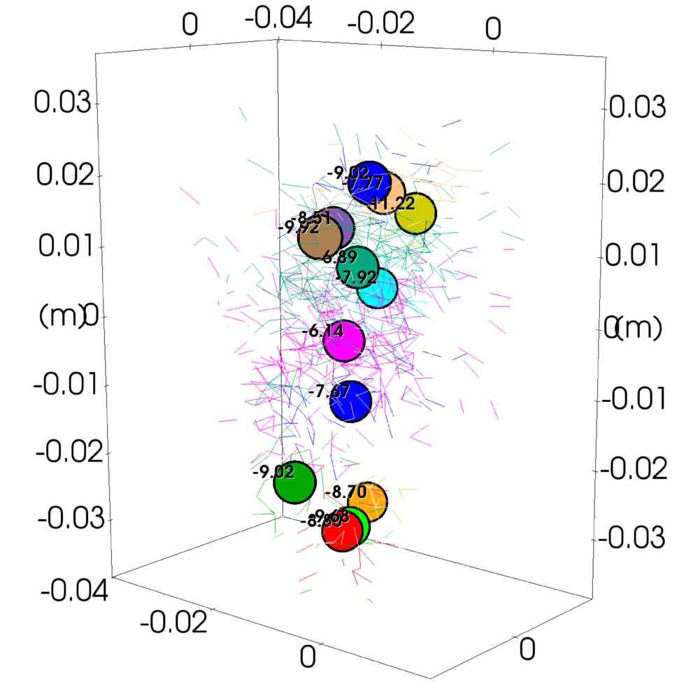
Example of clustered broken bonds (colored lines) and the final AE events (colored circles) with their event magnitudes.
For a detailed look at the underlying algorithm, please refer to the source code.
Activating the algorithm within Yade
The simulation of AE is available as part of Yade’s Jointed Cohesive Frictional particle model (JCFpm) . As such, your simulation needs to make use of JCFpmMat , JCFpmPhys , and Law2_ScGeom_JCFpmPhys
Your material assignment and engines list might look something like this:
       JCFmat = O.materials.append(JCFpmMat(young=young, cohesion=cohesion,
               density=density, frictionAngle=radians(finalFricDegree),
               tensileStrength=sigmaT, poisson=poisson, label='JCFmat',
               jointNormalStiffness=2.5e6,jointShearStiffness=1e6,jointCohesion=1e6))

       O.engines=[
                       ForceResetter(),
                       InsertionSortCollider([Bo1_Box_Aabb(),Bo1_Sphere_Aabb
                               ,Bo1_Facet_Aabb()]),
                       InteractionLoop(
                               [Ig2_Sphere_Sphere_ScGeom(), Ig2_Facet_Sphere_ScGeom()],
                               [Ip2_FrictMat_FrictMat_FrictPhys(),
                                       Ip2_JCFpmMat_JCFpmMat_JCFpmPhys( \
                                               xSectionWeibullScaleParameter=xSectionScale,
                                               xSectionWeibullShapeParameter=xSectionShape,
                                               weibullCutOffMin=weibullCutOffMin,
                                               weibullCutOffMax=weibullCutOffMax)],
                               [Law2_ScGeom_JCFpmPhys_JointedCohesiveFrictionalPM(\
                                       recordCracks=True, recordMoments=True,
                                       Key=identifier,label='interactionLaw'),
                               Law2_ScGeom_FrictPhys_CundallStrack()]
),

           GlobalStiffnessTimeStepper(),
           VTKRecorder(recorders=['jcfpm','cracks','facets','moments'] \
                               ,Key=identifier,label='vtk'),
                       NewtonIntegrator(damping=0.4)
       ]
Most of this simply enables JCFpm as usual, the AE relevant commands are:
Law2_ScGeom_JCFpmPhys_JointedCohesiveFrictionalPM(...  recordMoments=True ...)
VTKRecorder(... recorders=[... 'moments' ...])
There are some other commands necessary for proper activation and use of the acoustic emissions algorithm:
clusterMoments tells Yade to cluster new broken interactions within the user set spatial radius as described above in the model description. This value is set to True by default.
momentRadiusFactor is \(\lambda\) from the above model description. The momentRadiusFactor changes the number of particle radii beyond the initial interaction that Yade computes the strain energy change. Additionally, Yade uses \(\lambda\) to seek additional broken bonds for clustering. This value is set to 5 by default ( [Hazzard2013] concluded that this value yields accurate strain energy change approximations for the total strain energy change of the system entire system).
neverErase allows old interactions to be stored in memory despite no longer affecting the simulation. This value must be set to True for stable operation of Yade’s AE cluster model.
Visualizing and post processing acoustic emissions
AE are visualized and post processed in a similar manner to JCFpm cracks. As long as recordMoments=True and recorder=[‘moments’] , the simulation will produce timestamped .vtu files for easy Paraview post processing. Within Paraview, the AE can be filtered according to magnitude, number of constitiuent interactions, and event time. fig-aeexample shows AE collected during a three point bending test and filtered according to magnitude and time
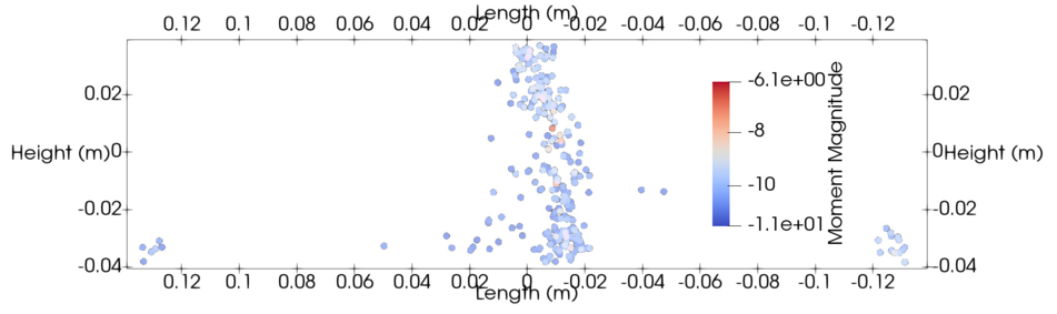
Example of AE simulated during three point bending test and filtered by magnitude and time.
Consideration of rock heterogeneity
[Caulk2018] and [Caulk2020] hypothesize that heterogeneous rock behavior depends on the distribution of interacting grain edge lengths. In support of the hypothesis, [Caulk2018] and [Caulk2020] show how rock heterogeneity can be modeled using cathodoluminescent grain imagery. A Weibull distribution is constructed based on the so called grain edge interaction length distribution. In Yade’s JCFpm , the Weibull distribution is used to modify the interaction strengths of contacting particles by correcting the interaction area \(A_{int}\):
where \(\alpha_w\) is the Weibull correction factor, which is distributed as shown in fig-weibullDist. The corresponding tensile strength distributions for various Weibull shape parameters are shown in fig-strengthDist. Note: a Weibull shape factor of \(\infty\) is equivalent to the unaugmented JCFpm model.
In Yade, the application of rock heterogeneity is as simple as passing a Weibull shape parameter to JCFpmPhys :
Ip2_JCFpmMat_JCFpmMat_JCFpmPhys(
        xSectionWeibullScaleParameter=xSectionScale,
        xSectionWeibullShapeParameter=xSectionShape,
        weibullCutOffMin=weibullCutOffMin,
        weibullCutOffMax=weibullCutOffMax)
where the xSectionWeibullShapeParameter is the desired Weibull shape parameter. The scale parameter can be assigned in similar fashion. If you want to control the minimum allowable correction factor, you can feed it weibullCutoffMin . The maximum correction factor can be controlled in similar fashion.
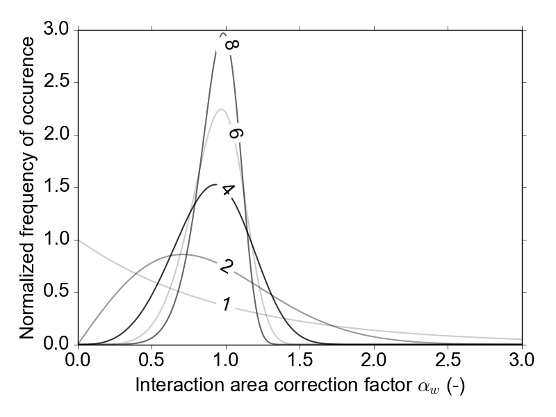
Weibull distributions for varying shape parameters used to generate \(\alpha_w\).
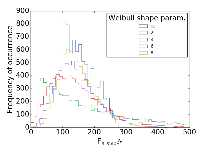
Maximum DEM particle bond tensile strength distributions for varying Weibull shape parameters.