DEM formulation

In this chapter, we mathematically describe general features of explicit DEM simulations, with some reference to Yade implementation of these algorithms. They are given roughly in the order as they appear in simulation; first, two particles might establish a new interaction, which consists in

1. detecting collision between particles;

2. creating new interaction and determining its properties (such as stiffness); they are either precomputed or derived from properties of both particles;

Then, for already existing interactions, the following is performed:

1. strain evaluation;

2. stress computation based on strains;

3. force application to particles in interaction.

This simplified description serves only to give meaning to the ordering of sections within this chapter. A more detailed description of this simulation loop is given later.

In this chapter we refer to kinematic variables of the contacts as ``strains``, although at this scale it is also common to speak of ``displacements``. Which semantic is more appropriate depends on the conceptual model one is starting from, and therefore it cannot be decided independently of specific problems. The reader familiar with displacements can mentaly replace normal strain and shear strain by normal displacement and shear displacement, respectively, without altering the meaning of what follows.

Collision detection

Generalities

Exact computation of collision configuration between two particles can be relatively expensive (for instance between Sphere and Facet). Taking a general pair of bodies $i$ and $j$ and their ``exact`` (In the sense of precision admissible by numerical implementation.) spatial predicates (called Shape in Yade) represented by point sets $P_i$, $P_j$ the detection generally proceeds in 2 passes:

1. fast collision detection using approximate predicate ${\tilde{P}}_i$ and ${\tilde{P}}_j$; they are pre-constructed in such a way as to abstract away individual features of $P_i$ and $P_j$ and satisfy the condition

   (1)$$\mathrm{\forall }\mathbf{x}\in R^3:x\in P_i\Rightarrow x\in {\tilde{P}}_i$$

   (likewise for $P_j$). The approximate predicate is called ``bounding volume’’ (Bound in Yade) since it bounds any particle’s volume from outside (by virtue of the implication). It follows that $(P_i\cap P_j)\ne \mathrm{\varnothing }\Rightarrow ({\tilde{P}}_i\cap {\tilde{P}}_j)\ne \mathrm{\varnothing }$ and, by applying modus tollens,

   (2)$$({\tilde{P}}_i\cap {\tilde{P}}_j)=\mathrm{\varnothing }\Rightarrow (P_i\cap P_j)=\mathrm{\varnothing }$$

   which is a candidate exclusion rule in the proper sense.

2. By filtering away impossible collisions in (2), a more expensive, exact collision detection algorithms can be run on possible interactions, filtering out remaining spurious couples $({\tilde{P}}_i\cap {\tilde{P}}_j)\ne \mathrm{\varnothing }\wedge (P_i\cap P_j)=\mathrm{\varnothing }$. These algorithms operate on $P_i$ and $P_j$ and have to be able to handle all possible combinations of shape types.

It is only the first step we are concerned with here.

Algorithms

Collision evaluation algorithms have been the subject of extensive research in fields such as robotics, computer graphics and simulations. They can be roughly divided in two groups:

Hierarchical algorithms

which recursively subdivide space and restrict the number of approximate checks in the first pass, knowing that lower-level bounding volumes can intersect only if they are part of the same higher-level bounding volume. Hierarchy elements are bounding volumes of different kinds: octrees [Jung1997], bounding spheres [Hubbard1996], k-DOP’s [Klosowski1998].

Flat algorithms

work directly with bounding volumes without grouping them in hierarchies first; let us only mention two kinds commonly used in particle simulations:

Sweep and prune

algorithm operates on axis-aligned bounding boxes, which overlap if and only if they overlap along all axes. These algorithms have roughly $\mathcal{O}(n\log n)$ complexity, where $n$ is number of particles as long as they exploit temporal coherence of the simulation.

Grid algorithms

represent continuous $R^3$ space by a finite set of regularly spaced points, leading to very fast neighbor search; they can reach the $\mathcal{O}(n)$ complexity [Munjiza1998] and recent research suggests ways to overcome one of the major drawbacks of this method, which is the necessity to adjust grid cell size to the largest particle in the simulation ([Munjiza2006], the ``multistep’’ extension).

Temporal coherence

expresses the fact that motion of particles in simulation is not arbitrary but governed by physical laws. This knowledge can be exploited to optimize performance.

Numerical stability of integrating motion equations dictates an upper limit on $\mathrm{\Delta }t$ (sect. Stability considerations) and, by consequence, on displacement of particles during one step. This consideration is taken into account in [Munjiza2006], implying that any particle may not move further than to a neighboring grid cell during one step allowing the $\mathcal{O}(n)$ complexity; it is also explored in the periodic variant of the sweep and prune algorithm described below.

On a finer level, it is common to enlarge ${\tilde{P}}_i$ predicates in such a way that they satisfy the (1) condition during several timesteps; the first collision detection pass might then be run with stride, speeding up the simulation considerably. The original publication of this optimization by Verlet [Verlet1967] used enlarged list of neighbors, giving this technique the name Verlet list. In general cases, however, where neighbor lists are not necessarily used, the term Verlet distance is employed.

Sweep and prune

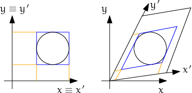
Let us describe in detail the sweep and prune algorithm used for collision detection in Yade (class InsertionSortCollider). Axis-aligned bounding boxes (Aabb) are used as ${\tilde{P}}_i$; each Aabb is given by lower and upper corner $\in R^3$ (in the following, ${\tilde{P}}_i^{x0}$, ${\tilde{P}}_i^{x1}$ are minimum/maximum coordinates of ${\tilde{P}}_i$ along the $x$-axis and so on). Construction of Aabb from various particle Shape’s (such as Sphere, Facet, Wall) is straightforward, handled by appropriate classes deriving form BoundFunctor (Bo1_Sphere_Aabb, Bo1_Facet_Aabb, …).

Presence of overlap of two Aabb’s can be determined from conjunction of separate overlaps of intervals along each axis (fig-sweep-and-prune):

$$({\tilde{P}}_i\cap {\tilde{P}}_j)\ne \mathrm{\varnothing }\iff \underset{w\in \{x,y,z\}}{\bigwedge }[(({\tilde{P}}_i^{w0},{\tilde{P}}_i^{w1})\cap ({\tilde{P}}_j^{w0},{\tilde{P}}_j^{w1}))\ne \mathrm{\varnothing }]$$

where $(a,b)$ denotes interval in $R$.

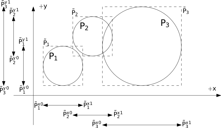
Sweep and prune algorithm (shown in 2D), where Aabb of each sphere is represented by minimum and maximum value along each axis. Spatial overlap of Aabb’s is present if they overlap along all axes. In this case, ${\tilde{P}}_1\cap {\tilde{P}}_2\ne \mathrm{\varnothing }$ (but note that $P_1\cap P_2=\mathrm{\varnothing }$) and ${\tilde{P}}_2\cap {\tilde{P}}_3\ne \mathrm{\varnothing }$.}

The collider keeps 3 separate lists (arrays) $L_w$ for each axis $w\in \{x,y,z\}$

$$L_w=\bigcup _i\{{\tilde{P}}_i^{w0},{\tilde{P}}_i^{w1}\}$$

where $i$ traverses all particles. $L_w$ arrays (sorted sets) contain respective coordinates of minimum and maximum corners for each Aabb (we call these coordinates bound in the following); besides bound, each of list elements further carries id referring to particle it belongs to, and a flag whether it is lower or upper bound.

In the initial step, all lists are sorted (using quicksort, average $\mathcal{O}(n\log n)$) and one axis is used to create initial interactions: the range between lower and upper bound for each body is traversed, while bounds in-between indicate potential Aabb overlaps which must be checked on the remaining axes as well.

At each successive step, lists are already pre-sorted. Inversions occur where a particle’s coordinate has just crossed another particle’s coordinate; this number is limited by numerical stability of simulation and its physical meaning (giving spatio-temporal coherence to the algorithm). The insertion sort algorithm swaps neighboring elements if they are inverted, and has complexity between $\mathcal{O}(n)$ and $\mathcal{O}(n^2)$, for pre-sorted and unsorted lists respectively. For our purposes, we need only to handle inversions, which by nature of the sort algorithm are detected inside the sort loop. An inversion might signify:

• overlap along the current axis, if an upper bound inverts (swaps) with a lower bound (i.e. that the upper bound with a higher coordinate was out of order in coming before the lower bound with a lower coordinate). Overlap along the other 2 axes is checked and if there is overlap along all axes, a new potential interaction is created.

• End of overlap along the current axis, if lower bound inverts (swaps) with an upper bound. If there is only potential interaction between the two particles in question, it is deleted.

• Nothing if both bounds are upper or both lower.

Aperiodic insertion sort

Let us show the sort algorithm on a sample sequence of numbers:

Elements are traversed from left to right; each of them keeps inverting (swapping) with neighbors to the left, moving left itself, until any of the following conditions is satisfied:

($\le$)	the sorting order with the left neighbor is correct, or
($||$)	the element is at the beginning of the sequence.

We start at the leftmost element (the current element is marked $\boxed{i}$)

It obviously immediately satisfies ($||$), and we move to the next element:

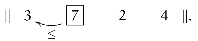
Condition ($\le$) holds, therefore we move to the right. The $\boxed{2}$ is not in order (violating ($\le$)) and two inversions take place; after that, ($||$) holds:

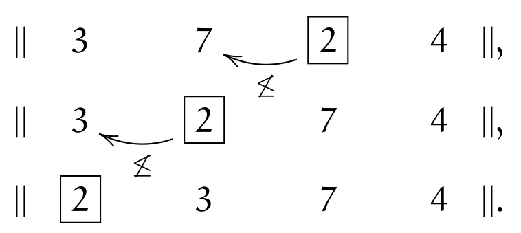
The last element $\boxed{4}$ first violates ($\le$), but satisfies it after one inversion

All elements having been traversed, the sequence is now sorted.

It is obvious that if the initial sequence were sorted, elements only would have to be traversed without any inversion to handle (that happens in $\mathcal{O}(n)$ time).

For each inversion during the sort in simulation, the function that investigates change in Aabb overlap is invoked, creating or deleting interactions.

The periodic variant of the sort algorithm is described in Periodic insertion sort algorithm, along with other periodic-boundary related topics.

Optimization with Verlet distances

As noted above, [Verlet1967] explored the possibility of running the collision detection only sparsely by enlarging predicates ${\tilde{P}}_i$.

In Yade, this is achieved by enlarging Aabb of particles by fixed relative length (or Verlet’s distance) in all dimensions $\mathrm{\Delta }L$ (InsertionSortCollider.sweepLength). Suppose the collider run last time at step $m$ and the current step is $n$. NewtonIntegrator tracks the cummulated distance traversed by each particle between $m$ and $n$ by comparing the current position with the reference position from time $n$ (Bound::refPos),

(3)$$L_{\mathrm{m}\mathrm{n}}=|X^n-X^m|$$

triggering the collider re-run as soon as one particle gives:

(4)$$L_{\mathrm{m}\mathrm{n}}>\mathrm{\Delta }L.$$

$\mathrm{\Delta }L$ is defined primarily by the parameter InsertionSortCollider.verletDist. It can be set directly by assigning a positive value, or indirectly by assigning negative value (which defines $\mathrm{\Delta }L$ in proportion of the smallest particle radius). In addition, InsertionSortCollider.targetInterv can be used to adjust $\mathrm{\Delta }L$ independently for each particle. Larger $\mathrm{\Delta }L$ will be assigned to the fastest ones, so that all particles would ideally reach the edge of their bounds after this “target” number of iterations. Results of using Verlet distance depend highly on the nature of simulation and choice of InsertionSortCollider.targetInterv. Adjusting the sizes independently for each particle is especially efficient if some parts of a problem have high-speed particles will others are not moving. If it is not the case, no significant gain should be expected as compared to targetInterv=0 (assigning the same $\mathrm{\Delta }L$ to all particles).

The number of particles and the number of available threads is also to be considered for choosing an appropriate Verlet’s distance. A larger distance will result in less time spent in the collider (which runs single-threaded) and more time in computing interactions (multi-threaded). Typically, large $\mathrm{\Delta }L$ will be used for large simulations with more than ${10}^5$ particles on multi-core computers. On the other hand simulations with less than ${10}^4$ particles on single processor will probably benefit from smaller $\mathrm{\Delta }L$. Users benchmarks may be found on Yade’s wiki (see e.g. https://yade-dem.org/wiki/Colliders_performace).

Creating interaction between particles

Collision detection described above is only approximate. Exact collision detection depends on the geometry of individual particles and is handled separately. In Yade terminology, the Collider creates only potential interactions; potential interactions are evaluated exactly using specialized algorithms for collision of two spheres or other combinations. Exact collision detection must be run at every timestep since it is at every step that particles can change their mutual position (the collider is only run sometimes if the Verlet distance optimization is in use). Some exact collision detection algorithms are described in Kinematic variables; in Yade, they are implemented in classes deriving from IGeomFunctor (prefixed with Ig2).

Besides detection of geometrical overlap (which corresponds to IGeom in Yade), there are also non-geometrical properties of the interaction to be determined (IPhys). In Yade, they are computed for every new interaction by calling a functor deriving from IPhysFunctor (prefixed with Ip2) which accepts the given combination of Material types of both particles.

Stiffnesses

Basic DEM interaction defines two stiffnesses: normal stiffness $K_N$ and shear (tangent) stiffness $K_T$. It is desirable that $K_N$ be related to fictitious Young’s modulus of the particles’ material, while $K_T$ is typically determined as a given fraction of computed $K_N$. The $K_T/K_N$ ratio determines macroscopic Poisson’s ratio of the arrangement, which can be shown by dimensional analysis: elastic continuum has two parameters ($E$ and $\nu$) and basic DEM model also has 2 parameters with the same dimensions $K_N$ and $K_T/K_N$; macroscopic Poisson’s ratio is therefore determined solely by $K_T/K_N$ and macroscopic Young’s modulus is then proportional to $K_N$ and affected by $K_T/K_N$.

Naturally, such analysis is highly simplifying and does not account for particle radius distribution, packing configuration and other possible parameters such as the interaction radius introduced later.

Normal stiffness

The algorithm commonly used in Yade computes normal interaction stiffness as stiffness of two springs in serial configuration with lengths equal to the sphere radii (fig-spheres-contact-stiffness).

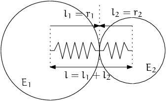
Series of 2 springs representing normal stiffness of contact between 2 spheres.

Let us define distance $l=l_1+l_2$, where $l_i$ are distances between contact point and sphere centers, which are initially (roughly speaking) equal to sphere radii. Change of distance between the sphere centers $\mathrm{\Delta }l$ is distributed onto deformations of both spheres $\mathrm{\Delta }l=\mathrm{\Delta }{l}_1+\mathrm{\Delta }{l}_2$ proportionally to their compliances. Displacement change $\mathrm{\Delta }{l}_i$ generates force $F_i=K_i\mathrm{\Delta }{l}_i$, where $K_i$ assures proportionality and has physical meaning and dimension of stiffness; $K_i$ is related to the sphere material modulus $E_i$ and some length ${\tilde{l}}_i$ proportional to $r_i$.

$$\begin{array}{rl}\mathrm{\Delta }l& =\mathrm{\Delta }{l}_1+\mathrm{\Delta }{l}_2\\ K_i& =E_i{\tilde{l}}_i\\ K_N\mathrm{\Delta }l& =F=F_1=F_2\\ K_N(\mathrm{\Delta }{l}_1+\mathrm{\Delta }{l}_2)& =F\\ K_N(\frac{F}{K_1}+\frac{F}{K_2})& =F\\ K_1^{-1}+K_2^{-1}& =K_N^{-1}\\ K_N& =\frac{K_1{K}_2}{K_1+K_2}\\ K_N& =\frac{E_1{\tilde{l}}_1{E}_2{\tilde{l}}_2}{E_1{\tilde{l}}_1+E_2{\tilde{l}}_2}\end{array}$$

The most used class computing interaction properties Ip2_FrictMat_FrictMat_FrictPhys uses ${\tilde{l}}_i=2r_i$.

Some formulations define an equivalent cross-section $A_{\mathrm{e}\mathrm{q}}$, which in that case appears in the ${\tilde{l}}_i$ term as $K_i=E_i{\tilde{l}}_i=E_i\frac{A_{\mathrm{e}\mathrm{q}}}{l_i}$. Such is the case for the concrete model (Ip2_CpmMat_CpmMat_CpmPhys), where $A_{\mathrm{e}\mathrm{q}}=min(r_1,r_2)$.

For reasons given above, no pretense about equality of particle-level $E_i$ and macroscopic modulus $E$ should be made. Some formulations, such as [Hentz2003], introduce parameters to match them numerically. This is not appropriate, in our opinion, since it binds those values to particular features of the sphere arrangement that was used for calibration.

Other parameters

Non-elastic parameters differ for various material models. Usually, though, they are averaged from the particles’ material properties, if it makes sense. For instance, Ip2_CpmMat_CpmMat_CpmPhys averages most quantities, while Ip2_FrictMat_FrictMat_FrictPhys computes internal friction angle as $\phi =min({\phi }_1,{\phi }_2)$ to avoid friction with bodies that are frictionless.

Kinematic variables

In the general case, mutual configuration of two particles has 6 degrees of freedom (DoFs) just like a beam in 3D space: both particles have 6 DoFs each, but the interaction itself is free to move and rotate in space (with both spheres) having 6 DoFs itself; then $12-6=6$. They are shown at fig-spheres-dofs.

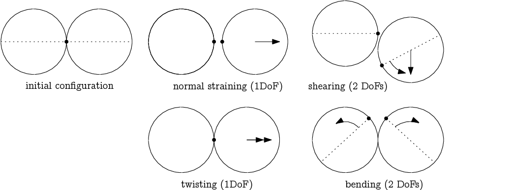
Degrees of freedom of configuration of two spheres. Normal motion appears if there is a difference of linear velocity along the interaction axis ($n$); shearing originates from the difference of linear velocities perpendicular to $n$ and from the part of ${\mathit{\omega }}_1+{\mathit{\omega }}_2$ perpendicular to $n$; twisting is caused by the part of ${\mathit{\omega }}_1-{\mathit{\omega }}_2$ parallel with $n$; bending comes from the part of ${\mathit{\omega }}_1-{\mathit{\omega }}_2$ perpendicular to $n$.

We will only describe normal and shear components of the relative movement in the following, leaving torsion and bending aside. The reason is that most constitutive laws for contacts do not use the latter two.

Normal deformation

Constants

Let us consider two spheres with initial centers $\overline{{\mathit{C}}_1}$, ${\overline{\mathit{C}}}_2$ and radii $r_1$, $r_2$ that enter into contact. The order of spheres within the contact is arbitrary and has no influence on the behavior. Then we define lengths

$$\begin{array}{rl}{d}_0& =|{\overline{\mathit{C}}}_2-{\overline{\mathit{C}}}_1|\\ d_1& =r_1+\frac{d_0-r_1-r_2}{2},& d_2& =d_0-d_1.\end{array}$$

These quantities are constant throughout the life of the interaction and are computed only once when the interaction is established. The distance $d_0$ is the reference distance and is used for the conversion of absolute displacements to dimensionless strain, for instance. It is also the distance where (for usual contact laws) there is neither repulsive nor attractive force between the spheres, whence the name equilibrium distance.

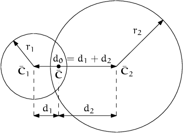
Geometry of the initial contact of 2 spheres; this case pictures spheres which already overlap when the contact is created (which can be the case at the beginning of a simulation) for the sake of generality. The initial contact point $\overline{\mathit{C}}$ is in the middle of the overlap zone.

Distances $d_1$ and $d_2$ define reduced (or expanded) radii of spheres; geometrical radii $r_1$ and $r_2$ are used only for collision detection and may not be the same as $d_1$ and $d_2$, as shown in fig. fig-sphere-sphere. This difference is exploited in cases where the average number of contacts between spheres should be increased, e.g. to influence the response in compression or to stabilize the packing. In such case, interactions will be created also for spheres that do not geometrically overlap based on the interaction radius $R_I$, a dimensionless parameter determining „non-locality“ of contact detection. For $R_I=1$, only spheres that touch are considered in contact; the general condition reads

(5)$$d_0\le R_I(r_1+r_2).$$

The value of $R_I$ directly influences the average number of interactions per sphere (percolation), which for some models is necessary in order to achieve realistic results. In such cases, Aabb (or ${\tilde{P}}_i$ predicates in general) must be enlarged accordingly (Bo1_Sphere_Aabb.aabbEnlargeFactor).

Contact cross-section

Some constitutive laws are formulated with strains and stresses (Law2_ScGeom_CpmPhys_Cpm, the concrete model described later, for instance); in that case, equivalent cross-section of the contact must be introduced for the sake of dimensionality. The exact definition is rather arbitrary; the CPM model (Ip2_CpmMat_CpmMat_CpmPhys) uses the relation

(6)$$A_{\mathrm{e}\mathrm{q}}=\pi min(r_1,r_2{)}^2$$

which will be used to convert stresses to forces, if the constitutive law used is formulated in terms of stresses and strains. Note that other values than $\pi$ can be used; it will merely scale macroscopic packing stiffness; it is only for the intuitive notion of a truss-like element between the particle centers that we choose $A_{\mathrm{e}\mathrm{q}}$ representing the circle area. Besides that, another function than $min(r_1,r_2)$ can be used, although the result should depend linearly on $r_1$ and $r_2$ so that the equation gives consistent results if the particle dimensions are scaled.

Variables

The following state variables are updated as spheres undergo motion during the simulation (as ${\mathit{C}}_1^{\circ }$ and ${\mathit{C}}_2^{\circ }$ change):

(7)$${\mathit{n}}^{\circ }=\frac{{\mathit{C}}_2^{\circ }-{\mathit{C}}_1^{\circ }}{|{\mathit{C}}_2^{\circ }-{\mathit{C}}_1^{\circ }|}\equiv \widehat{{\mathit{C}}_2^{\circ }-{\mathit{C}}_1^{\circ }}$$

and

(8)$${\mathit{C}}^{\circ }={\mathit{C}}_1^{\circ }+(d_1-\frac{d_0-|{\mathit{C}}_2^{\circ }-{\mathit{C}}_1^{\circ }|}{2})\mathit{n}.$$

The contact point ${\mathit{C}}^{\circ }$ is always in the middle of the spheres’ overlap zone (even if the overlap is negative, when it is in the middle of the empty space between the spheres). The contact plane is always perpendicular to the contact plane normal ${\mathit{n}}^{\circ }$ and passes through ${\mathit{C}}^{\circ }$.

Normal displacement and strain can be defined as

$$\begin{array}{rl}{u}_N& =|{\mathit{C}}_2^{\circ }-{\mathit{C}}_1^{\circ }|-d_0,\\ {\epsilon }_N& =\frac{u_N}{d_0}=\frac{|{\mathit{C}}_2^{\circ }-{\mathit{C}}_1^{\circ }|}{d_0}-1.\end{array}$$

Since $u_N$ is always aligned with $\mathit{n}$, it can be stored as a scalar value multiplied by $\mathit{n}$ if necessary.

For massively compressive simulations, it might be beneficial to use the logarithmic strain, such that the strain tends to $-\mathrm{\infty }$ (rather than $-1$) as centers of both spheres approach. Otherwise, repulsive force would remain finite and the spheres could penetrate through each other. Therefore, we can adjust the definition of normal strain as follows:

$$\begin{array}{r}{\epsilon }_N=\{\begin{array}{ll}\log \left(\frac{|{\mathit{C}}_2^{\circ }-{\mathit{C}}_1^{\circ }|}{d_0}\right)& \text{if }|{\mathit{C}}_2^{\circ }-{\mathit{C}}_1^{\circ }|<d_0\\ \frac{|{\mathit{C}}_2^{\circ }-{\mathit{C}}_1^{\circ }|}{d_0}-1& \text{otherwise.}\end{array}\end{array}$$

Such definition, however, has the disadvantage of effectively increasing rigidity (up to infinity) of contacts, requiring $\mathrm{\Delta }t$ to be adjusted, lest the simulation becomes unstable. Such dynamic adjustment is possible using a stiffness-based time-stepper (GlobalStiffnessTimeStepper in Yade).

Shear deformation

In order to keep ${\mathit{u}}_T$ consistent (e.g. that ${\mathit{u}}_T$ must be constant if two spheres retain mutually constant configuration but move arbitrarily in space), then either ${\mathit{u}}_T$ must track spheres’ spatial motion or must (somehow) rely on sphere-local data exclusively.

Geometrical meaning of shear strain is shown in fig-shear-2d.

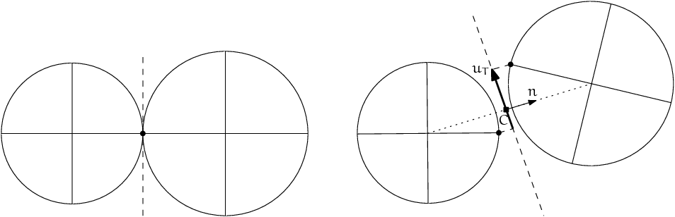
Evolution of shear displacement ${\mathit{u}}_T$ due to mutual motion of spheres, both linear and rotational. Left configuration is the initial contact, right configuration is after displacement and rotation of one particle.

The classical incremental algorithm is widely used in DEM codes and is described frequently ([Luding2008], [Alonso2004]). Yade implements this algorithm in the ScGeom class. At each step, shear displacement ${\mathit{u}}_T$ is updated; the update increment can be decomposed in 2 parts: motion of the interaction (i.e. $\mathit{C}$ and $\mathit{n}$) in global space and mutual motion of spheres.

1. Contact moves dues to changes of the spheres’ positions ${\mathit{C}}_1$ and ${\mathit{C}}_2$, which updates current ${\mathit{C}}^{\circ }$ and ${\mathit{n}}^{\circ }$ as per (8) and (7). ${\mathit{u}}_T^{-}$ is perpendicular to the contact plane at the previous step ${\mathit{n}}^{-}$ and must be updated so that ${\mathit{u}}_T^{-}+(\mathrm{\Delta }{\mathit{u}}_T)={\mathit{u}}_T^{\circ }\perp {\mathit{n}}^{\circ }$; this is done by perpendicular projection to the plane first (which might decrease $|{\mathit{u}}_T|$) and adding what corresponds to spatial rotation of the interaction instead:

   $$\begin{array}{rl}(\mathrm{\Delta }{\mathit{u}}_T{)}_1& =-{\mathit{u}}_T^{-}\times ({\mathit{n}}^{-}\times {\mathit{n}}^{\circ })\\ (\mathrm{\Delta }{\mathit{u}}_T{)}_2& =-{\mathit{u}}_T^{-}\times (\frac{\mathrm{\Delta }t}{2}{\mathit{n}}^{\circ }\cdot ({\mathit{\omega }}_1^{\ominus }+{\mathit{\omega }}_2^{\ominus })){\mathit{n}}^{\circ }\end{array}$$

2. Mutual movement of spheres, using only its part perpendicular to ${\mathit{n}}^{\circ }$; ${\mathit{v}}_{12}$ denotes mutual velocity of spheres at the contact point:

   $$\begin{array}{rl}{\mathit{v}}_{12}& =({\mathit{v}}_2^{\ominus }+{\mathit{\omega }}_2^{\ominus }\times (-d_2{\mathit{n}}^{\circ }))-({\mathit{v}}_1^{\ominus }+{\mathit{\omega }}_1^{\ominus }\times (d_1{\mathit{n}}^{\circ }))\\ {\mathit{v}}_{12}^{\perp }& ={\mathit{v}}_{12}-({\mathit{n}}^{\circ }\cdot {\mathit{v}}_{12}){\mathit{n}}^{\circ }\\ (\mathrm{\Delta }{\mathit{u}}_T{)}_3& =-\mathrm{\Delta }t{\mathit{v}}_{12}^{\perp }\end{array}$$

Finally, we compute

$${\mathit{u}}_T^{\circ }={\mathit{u}}_T^{-}+(\mathrm{\Delta }{\mathit{u}}_T{)}_1+(\mathrm{\Delta }{\mathit{u}}_T{)}_2+(\mathrm{\Delta }{\mathit{u}}_T{)}_3.$$

Contact model (example)

The kinematic variables of an interaction are used to determine the forces acting on both spheres via a constitutive law. In DEM generally, some constitutive laws are expressed using strains and stresses while others prefer displacement/force formulation. The law described here falls in the latter category.

The constitutive law presented here is the most common in DEM, originally proposed by Cundall. While the kinematic variables are described in the previous section regardless of the contact model, the force evaluation depends on the nature of the material being modeled. The constitutive law presented here is the simplest non-cohesive elastic-frictional contact model, which Yade implements in Law2_ScGeom_FrictPhys_CundallStrack (all constitutive laws derive from base class LawFunctor).

When new contact is established (discussed in Engines) it has its properties (IPhys) computed from Materials associated with both particles. In the simple case of frictional material FrictMat, Ip2_FrictMat_FrictMat_FrictPhys creates a new FrictPhys instance, which defines normal stiffness $K_N$, shear stiffness $K_T$ and friction angle $\phi$.

At each step, given normal and shear displacements $u_N$, ${\mathit{u}}_T$, normal and shear forces are computed (if $u_N>0$, the contact is deleted without generating any forces):

$$\begin{array}{rl}{\mathit{F}}_N& =K_N{u}_N\mathit{n},\\ {\mathit{F}}_T^t& =K_T{\mathit{u}}_T\end{array}$$

where ${\mathit{F}}_N$ is normal force and ${\mathit{F}}_T^t$ is trial shear force. A simple non-associated stress return algorithm is applied to compute final shear force

$$\begin{array}{r}{\mathit{F}}_T=\{\begin{array}{ll}{\mathit{F}}_T^t\frac{|{\mathit{F}}_N|\tan \phi }{|{\mathit{F}}_T^t|}& \text{if }|{\mathit{F}}_T^t|>|{\mathit{F}}_N|\tan \phi ,\\ {\mathit{F}}_T^t& \text{otherwise.}\end{array}\end{array}$$

Summary force $\mathit{F}={\mathit{F}}_N+{\mathit{F}}_T$ is then applied to both particles – each particle accumulates forces and torques acting on it in the course of each step. Because the force computed acts at contact point $\mathit{C}$, which is difference from spheres’ centers, torque generated by $\mathit{F}$ must also be considered.

$$\begin{array}{rlrl}{\mathit{F}}_1& +=\mathit{F}& {\mathit{F}}_2& +=-\mathit{F}\\ {\mathit{T}}_1& +=d_1(-\mathit{n})\times \mathit{F}& {\mathit{T}}_2& +=d_2\mathit{n}\times \mathit{F}.\end{array}$$

Motion integration

Each particle accumulates generalized forces (forces and torques) from the contacts in which it participates. These generalized forces are then used to integrate motion equations for each particle separately; therefore, we omit $i$ indices denoting the $i$-th particle in this section.

The customary leapfrog scheme (also known as the Verlet scheme) is used, with some adjustments for rotation of non-spherical particles, as explained below. The “leapfrog” name comes from the fact that even derivatives of position/orientation are known at on-step points, whereas odd derivatives are known at mid-step points. Let us recall that we use $a^{-}$, $a^{\circ }$, $a^{+}$ for on-step values of $a$ at $t-\mathrm{\Delta }t$, $t$ and $t+\mathrm{\Delta }t$ respectively; and $a^{\ominus }$, $a^{\oplus }$ for mid-step values of $a$ at $t-\mathrm{\Delta }t/2$, $t+\mathrm{\Delta }t/2$.

Described integration algorithms are implemented in the NewtonIntegrator class in Yade.

Position

Integrating motion consists in using current acceleration ${\ddot{\mathit{u}}}^{\circ }$ on a particle to update its position from the current value ${\mathit{u}}^{\circ }$ to its value at the next timestep ${\mathit{u}}^{+}$. Computation of acceleration, knowing current forces $\mathit{F}$ acting on the particle in question and its mass $m$, is simply

$${\ddot{\mathit{u}}}^{\circ }=\mathit{F}/m.$$

Using the 2nd order finite difference with step $\mathrm{\Delta }t$, we obtain

$${\ddot{\mathit{u}}}^{\circ }\cong \frac{{\mathit{u}}^{-}-2{\mathit{u}}^{\circ }+{\mathit{u}}^{+}}{\mathrm{\Delta }{t}^2}$$

from which we express

$$\begin{array}{rl}{\mathit{u}}^{+}& =2{\mathit{u}}^{\circ }-{\mathit{u}}^{-}+{\ddot{\mathit{u}}}^{\circ }\mathrm{\Delta }{t}^2=\\ & ={\mathit{u}}^{\circ }+\mathrm{\Delta }t\underset{(†)}{\underbrace{(\frac{{\mathit{u}}^{\circ }-{\mathit{u}}^{-}}{\mathrm{\Delta }t}+{\ddot{\mathit{u}}}^{\circ }\mathrm{\Delta }t)}}.\end{array}$$

Typically, ${\mathit{u}}^{-}$ is already not known (only ${\mathit{u}}^{\circ }$ is); we notice, however, that

$${\dot{\mathit{u}}}^{\ominus }\simeq \frac{{\mathit{u}}^{\circ }-{\mathit{u}}^{-}}{\mathrm{\Delta }t},$$

i.e. the mean velocity during the previous step, which is known. Plugging this approximate into the $(†)$ term, we also notice that mean velocity during the current step can be approximated as

$${\dot{\mathit{u}}}^{\oplus }\simeq {\dot{\mathit{u}}}^{\ominus }+{\ddot{\mathit{u}}}^{\circ }\mathrm{\Delta }t,$$

which is $(†)$; we arrive finally at

$${\mathit{u}}^{+}={\mathit{u}}^{\circ }+\mathrm{\Delta }t({\dot{\mathit{u}}}^{\ominus }+{\ddot{\mathit{u}}}^{\circ }\mathrm{\Delta }t).$$

The algorithm can then be written down by first computing current mean velocity ${\dot{\mathit{u}}}^{\oplus }$ which we need to store for the next step (just as we use its old value ${\dot{\mathit{u}}}^{\ominus }$ now), then computing the position for the next time step ${\mathit{u}}^{+}$:

$$\begin{array}{rl}{\dot{\mathit{u}}}^{\oplus }& ={\dot{\mathit{u}}}^{\ominus }+{\ddot{\mathit{u}}}^{\circ }\mathrm{\Delta }t\\ {\mathit{u}}^{+}& ={\mathit{u}}^{\circ }+{\dot{\mathit{u}}}^{\oplus }\mathrm{\Delta }t.\end{array}$$

Positions are known at times $i\mathrm{\Delta }t$ (if $\mathrm{\Delta }t$ is constant) while velocities are known at $i\mathrm{\Delta }t+\frac{\mathrm{\Delta }t}{2}$. The fact that they interleave (jump over each other) in such way gave rise to the colloquial name “leapfrog” scheme.

Orientation

YADE has three different algorithms for integrating the rotational motion of non-spherical particles and one for spherical particles.

Orientation (spherical)

Updating particle orientation $q^{\circ }$ proceeds in an analogous way to position update. First, we compute current angular acceleration ${\dot{\mathit{\omega }}}^{\circ }$ from known current torque $\mathit{T}$. For spherical particles where the inertia tensor is diagonal in any orientation (therefore also in current global orientation), satisfying ${\mathit{I}}_{11}={\mathit{I}}_{22}={\mathit{I}}_{33}$, we can write

$${\dot{\mathit{\omega }}}_i^{\circ }={\mathit{T}}_i/{\mathit{I}}_{11},$$

We use the same approximation scheme, obtaining an equation analogous to (9)

$${\mathit{\omega }}^{\oplus }={\mathit{\omega }}^{\ominus }+\mathrm{\Delta }t{\dot{\mathit{\omega }}}^{\circ }.$$

The quaternion $\mathrm{\Delta }q$ representing rotation vector ${\mathit{\omega }}^{\oplus }\mathrm{\Delta }t$ is constructed, i.e. such that

$$\begin{array}{rl}(\mathrm{\Delta }q{)}_{\vartheta }& =|{\mathit{\omega }}^{\oplus }|,\\ (\mathrm{\Delta }q{)}_{\mathit{u}}& =\widehat{{\mathit{\omega }}^{\oplus }}\end{array}$$

Finally, we compute the next orientation $q^{+}$ by rotation composition

$$q^{+}=\mathrm{\Delta }q{q}^{\circ }.$$

Orientation (aspherical)

Integrating the rotation of aspherical particles is considerably more complicated than their position, as their local reference frame is not inertial. Rotation of rigid body in the local frame, where inertia matrix $\mathit{I}$ is diagonal, is described in the continuous form by Euler’s equations ($i\in \{1,2,3\}$ and $i$, $j$, $k$ are subsequent indices):

$${\mathit{T}}_i={\mathit{I}}_{ii}{\dot{\mathit{\omega }}}_i+({\mathit{I}}_{kk}-{\mathit{I}}_{jj}){\mathit{\omega }}_j{\mathit{\omega }}_k.$$

Due to the presence of both $\mathit{\omega }$ and $\dot{\mathit{\omega }}$, the equation cannot be solved using the standard leapfrog algorithm (that was the case for translational motion and also for the spherical bodies’ rotation where this equation reduced to $\mathit{T}=\mathit{I}\dot{\mathit{\omega }}$). The different integration algorithms for non-spherical particles can be selected using the NewtonIntegrator.rotAlgorithm argument of the NewtonIntegrator.

The default algorithm and the most accurate one was proposed by [delValle2023]. The algorithm uses a leapfrog formulation that conserves the norm of the quaternion. [Omelyan1998], a more general version of [Omelyan1999] algorithm, is also implemented. Previously, YADE used the algorithm described by [Allen1989] (pg. 84–89) and designed by [Fincham1992] for molecular dynamics problems; it consists of extending the leapfrog algorithm by mid-step/on-step estimators of quantities known at on-step/mid-step points in the basic formulation. Although it has received criticism and more precise algorithms were known ([Omelyan1999], [Neto2006], [Johnson2008]), this algorithm is implemented in Yade for its relative simplicity.

Each body has its local coordinate system based on the principal axes of inertia for that body. We use $\tilde{\bullet }$ to denote vectors in local coordinates. The orientation of the local system is given by the current particle’s orientation $q^{\circ }$ as a quaternion; this quaternion can be expressed as the (current) rotation matrix $\mathit{A}$. Therefore, every vector $\mathit{a}$ is transformed as $\tilde{\mathit{a}}=q\mathit{a}{q}^{\ast }=\mathit{A}\mathit{a}$. Since $\mathit{A}$ is a rotation (orthogonal) matrix, the inverse rotation ${\mathit{A}}^{-1}={\mathit{A}}^T$.

For a given particle, we know

• ${\tilde{\mathit{I}}}^{\circ }$ (constant) inertia matrix; diagonal, since in local, principal coordinates,

• ${\mathit{T}}^{\circ }$ external torque,

• $q^{\circ }$ current orientation (and its equivalent rotation matrix $\mathit{A}$),

• ${\mathit{\omega }}^{\ominus }$ mid-step angular velocity,

• ${\mathit{L}}^{\ominus }$ mid-step angular momentum; this is an auxiliary variable needed in Fincham’s algorithm. It will be zero in the initial step.

SPIRAL Algorithm ([delValle2023])

Our goal is to compute new values of the latter three, that is, ${\mathit{L}}^{\oplus }$, $q^{+}$, ${\mathit{\omega }}^{\oplus }$. We first estimate the current angular velocity:

$$\begin{array}{rl}{\mathit{K}}_{\mathbf{1}}& =dt\dot{\tilde{\mathit{\omega }}}({\tilde{\mathit{\omega }}}^{\ominus },{\tilde{\mathit{T}}}^{\circ }),\\ {\mathit{K}}_{\mathbf{2}}& =dt\dot{\tilde{\mathit{\omega }}}({\tilde{\mathit{\omega }}}^{\ominus }+{\mathit{K}}_{\mathbf{1}},{\tilde{\mathit{T}}}^{\circ }),\\ {\mathit{K}}_{\mathbf{3}}& =dt\dot{\tilde{\mathit{\omega }}}({\tilde{\mathit{\omega }}}^{\ominus }+\frac{1}{4}({\mathit{K}}_{\mathbf{1}}+{\mathit{K}}_{\mathbf{2}}),{\tilde{\mathit{T}}}^{\circ }),\\ {\tilde{\mathit{\omega }}}^{\oplus }& ={\tilde{\mathit{\omega }}}^{\ominus }+\frac{1}{6}({\mathit{K}}_{\mathbf{1}}+{\mathit{K}}_{\mathbf{2}}+4{\mathit{K}}_{\mathbf{3}}),\end{array}$$

where $\widetilde{\dot{\mathit{\omega }}}$ is given by Euler’s equation of motion, and we treat it as a function of angular velocity and torque. This way of integrating the angular velocity is similar to the Strong Stability Preserving Runge-Kutta-3 (SSPRK3) scheme but keeps the torque constant during the time step to avoid costly force recalculations. Then, we compute $q^{+}$, using $q^{\circ }$ and ${\tilde{\mathit{\omega }}}^{\oplus }$:

$$\begin{array}{rl}{q}^{+}& =q^{\circ }(\cos \vartheta +\frac{{\tilde{\mathit{\omega }}}^{\oplus }}{|{\tilde{\mathit{\omega }}}^{\oplus }|}\sin \vartheta ),\\ \vartheta & =\frac{dt}{2}|{\tilde{\mathit{\omega }}}^{\oplus }|,\end{array}$$

where the quantity inside the parenthesis is a quaternion represented by its scalar part and its imaginary (vectorial) part. The algorithm offers a third-order approximation for both the quaternion and angular velocity calculations. As this formulation conserves the norm of the quaternion, it does not need to be normalized every time step. It is normalized every NewtonIntegrator.normalizeEvery steps. To finish, we compute the angular velocity and momentum in the global reference frame:

$$\begin{array}{rl}{\mathit{\omega }}^{\oplus }& ={\mathit{A}}^{-1}{\tilde{\mathit{\omega }}}^{\oplus }.\\ {\mathit{L}}^{\oplus }& ={\mathit{A}}^{-1}({\tilde{\mathit{I}}}^{\circ }{\tilde{\mathit{\omega }}}^{\oplus }).\end{array}$$

Omelyan Algorithm

[Omelyan1999] algorithm is also a leapfrog formulation. However, note that in a leapfrog formulation, we require the mid-step velocity and the current derivative of the velocity. But, in the case of Euler’s equation, the current angular acceleration depends on the current angular velocity, which is unknown. Then, Omelyan proposes to interpolate the current angular velocity product as ${\tilde{\mathit{\omega }}}_j^{\circ }{\tilde{\mathit{\omega }}}_k^{\circ }\approx \frac{1}{2}({\tilde{\mathit{\omega }}}_j^{\ominus }{\tilde{\mathit{\omega }}}_k^{\ominus }+{\tilde{\mathit{\omega }}}_j^{\oplus }{\tilde{\mathit{\omega }}}_k^{\oplus })$. This leads to a non-linear system of equations that can efficiently be solved by iteration:

$$\begin{array}{rl}{\tilde{\mathit{\omega }}}_{i,n+1}^{\oplus }& ={\tilde{\mathit{\omega }}}_i^{\ominus }+\frac{dt}{{\mathit{I}}_{ii}}({\tilde{\mathit{T}}}_i^{\circ }-\frac{1}{2}({\mathit{I}}_{kk}-{\mathit{I}}_{jj})({\tilde{\mathit{\omega }}}_j^{\ominus }{\tilde{\mathit{\omega }}}_k^{\ominus }+{\tilde{\mathit{\omega }}}_{j,n}^{\oplus }{\tilde{\mathit{\omega }}}_{k,n}^{\oplus })).\end{array}$$

Then, we can compute the orientation of the particle with

$$\begin{array}{r}{q}^{+}=\frac{1-\frac{d{t}^2}{16}|{\tilde{\mathit{\omega }}}^{\oplus }{|}^2}{1+\frac{d{t}^2}{16}|{\tilde{\mathit{\omega }}}^{\oplus }{|}^2}{q}^{\circ }+\frac{dt{\dot{q}}^{\circ }}{1+\frac{d{t}^2}{16}|{\tilde{\mathit{\omega }}}^{\oplus }{|}^2}.\end{array}$$

The norm-conserving derivative of a quaternion can be calculated as

$$\begin{array}{r}{\dot{q}}^{\circ }=\frac{1}{2}{q}^{\circ }{\tilde{\omega }}^{\oplus },\end{array}$$

where ${\tilde{\omega }}^{\oplus }$ is a quaternion with a real part equal to zero and an imaginary part equal to the angular velocity. This can also be written as

$$\begin{array}{rl}\left(\begin{array}{c}{\dot{q}}_w^{\circ }\\ {\dot{q}}_x^{\circ }\\ {\dot{q}}_y^{\circ }\\ {\dot{q}}_z^{\circ }\end{array}\right)& =\frac{1}{2}\left(\begin{array}{cccc}{q}_w^{\circ }& -q_x^{\circ }& -q_y^{\circ }& -q_z^{\circ }\\ q_x^{\circ }& q_w^{\circ }& -q_z^{\circ }& q_y^{\circ }\\ q_y^{\circ }& q_z^{\circ }& q_w^{\circ }& -q_x^{\circ }\\ q_z^{\circ }& -q_y^{\circ }& q_x^{\circ }& q_w^{\circ }\end{array}\right)\left(\begin{array}{c}0\\ {\tilde{\mathit{\omega }}}_x^{\circ }\\ {\tilde{\mathit{\omega }}}_y^{\circ }\\ {\tilde{\mathit{\omega }}}_z^{\circ }\end{array}\right),\end{array}$$

In the same way as the last algorithm, it is a third-order approximation, and the formulation is orthonormal, meaning that the norm of the quaternion is conserved. However, this formulation is numerically not as stable as the previous one.

Fincham Algorithm

Unlike the other two algorithms, [Fincham1992] does not conserve the norm of the quaternion. Then, NewtonIntegrator.normalizeEvery has no effect over this algorithm. This algorithm is second-order. The algorithm goes as follows: first, we estimate the current angular momentum and compute the current local angular velocity:

$$\begin{array}{rlrl}{\mathit{L}}^{\circ }& ={\mathit{L}}^{\ominus }+{\mathit{T}}^{\circ }\frac{\mathrm{\Delta }t}{2},& {\tilde{\mathit{L}}}^{\circ }& =\mathit{A}{\mathit{L}}^{\circ },\\ {\mathit{L}}^{\oplus }& ={\mathit{L}}^{\ominus }+{\mathit{T}}^{\circ }\mathrm{\Delta }t,& {\tilde{\mathit{L}}}^{\oplus }& =\mathit{A}{\mathit{L}}^{\oplus },\\ {\tilde{\mathit{\omega }}}^{\circ }& ={\tilde{\mathit{I}}}^{\circ }{}^{-1}{\tilde{\mathit{L}}}^{\circ },\\ {\tilde{\mathit{\omega }}}^{\oplus }& ={\tilde{\mathit{I}}}^{\circ }{}^{-1}{\tilde{\mathit{L}}}^{\oplus }.\end{array}$$

Then, we evaluate ${\dot{q}}^{\oplus }$ from $q^{\oplus }$ and ${\tilde{\mathit{\omega }}}^{\oplus }$ in the same way as in (10) but shifted by $\mathrm{\Delta }t/2$ ahead. Then we can finally compute the desired values

$$\begin{array}{rl}{q}^{+}& =q^{\circ }+{\dot{q}}^{\oplus }\mathrm{\Delta }t,\\ {\mathit{\omega }}^{\oplus }& ={\mathit{A}}^{-1}{\tilde{\mathit{\omega }}}^{\oplus }.\end{array}$$

Clumps (rigid aggregates)

DEM simulations frequently make use of rigid aggregates of particles to model complex shapes [Price2007] called clumps, typically composed of many spheres. Dynamic properties of clumps are computed from the properties of its members:

• For non-overlapping clump members the clump’s mass $m_c$ is summed over members, the inertia tensor ${\mathbf{I}}_c$ is computed using the parallel axes theorem: ${\mathbf{I}}_c=\sum _i(m_i\ast d_i^2+I_i)$, where $m_i$ is the mass of clump member $i$, $d_i$ is the distance from center of clump member $i$ to clump’s centroid and $I_i$ is the inertia tensor of the clump member $i$.

• For overlapping clump members the clump’s mass $m_c$ is summed over cells using a regular grid spacing inside axis-aligned bounding box (Aabb) of the clump, the inertia tensor is computed using the parallel axes theorem: ${\mathbf{I}}_c=\sum _j(m_j\ast d_j^2+I_j)$, where $m_j$ is the mass of cell $j$, $d_j$ is the distance from cell center to clump’s centroid and $I_j$ is the inertia tensor of the cell $j$.

Local axes are oriented such that they are principal and inertia tensor is diagonal and clump’s orientation is changed to compensate rotation of the local system, as to not change the clump members’ positions in global space. Initial positions and orientations of all clump members in local coordinate system are stored.

In Yade (class Clump), clump members behave as stand-alone particles during simulation for purposes of collision detection and contact resolution, except that they have no contacts created among themselves within one clump. It is at the stage of motion integration that they are treated specially. Instead of integrating each of them separately, forces/torques on those particles ${\mathit{F}}_i$, ${\mathit{T}}_i$ are converted to forces/torques on the clump itself. Let us denote $r_i$ relative position of each particle with regards to clump’s centroid, in global orientation. Then summary force and torque on the clump are

$$\begin{array}{rl}{\mathit{F}}_c& =\sum F_i,\\ {\mathit{T}}_c& =\sum r_i\times F_i+T_i.\end{array}$$

Motion of the clump is then integrated, using aspherical rotation integration. Afterwards, clump members are displaced in global space, to keep their initial positions and orientations in the clump’s local coordinate system. In such a way, relative positions of clump members are always the same, resulting in the behavior of a rigid aggregate.

Numerical damping

In simulations of quasi-static phenomena, it it desirable to dissipate kinetic energy of particles. Since most constitutive laws (including Law_ScGeom_FrictPhys_Basic shown above, Contact model (example)) do not include velocity-based damping (such as one in [Addetta2001]), it is possible to use artificial numerical damping. The formulation is described in [Pfc3dManual30], although our version is slightly adapted. The basic idea is to decrease forces which increase the particle velocities and vice versa by $(\mathrm{\Delta }F{)}_d$, comparing the current acceleration sense and particle velocity sense. This is done by component, which makes the damping scheme clearly non-physical, as it is not invariant with respect to coordinate system rotation; on the other hand, it is very easy to compute. Cundall proposed the form (we omit particle indices $i$ since it applies to all of them separately):

$$\frac{(\mathrm{\Delta }\mathit{F}{)}_{dw}}{{\mathit{F}}_w}=-{\lambda }_d\mathrm{sgn}({\mathit{F}}_w{\dot{\mathit{u}}}_w^{\ominus }),w\in \{x,y,z\}$$

where ${\lambda }_d$ is the damping coefficient. This formulation has several advantages [Hentz2003]:

• it acts on forces (accelerations), not constraining uniform motion;

• it is independent of eigenfrequencies of particles, they will be all damped equally;

• it needs only the dimensionless parameter ${\lambda }_d$ which does not have to be scaled.

In Yade, we use the adapted form

(11)$$\frac{(\mathrm{\Delta }\mathit{F}{)}_{dw}}{{\mathit{F}}_w}=-{\lambda }_d\mathrm{sgn}{\mathit{F}}_w\underset{\simeq {\dot{u}}_w^{\circ }}{\underbrace{({\dot{u}}_w^{\ominus }+\frac{{\ddot{\mathit{u}}}_w^{\circ }\mathrm{\Delta }t}{2})}},$$

where we replaced the previous mid-step velocity ${\dot{u}}^{\ominus }$ by its on-step estimate in parentheses. This is to avoid locked-in forces that appear if the velocity changes its sign due to force application at each step, i.e. when the particle in question oscillates around the position of equilibrium with $2\mathrm{\Delta }t$ period.

In Yade, damping (11) is implemented in the NewtonIntegrator engine; the damping coefficient ${\lambda }_d$ is NewtonIntegrator.damping.

Stability considerations

Critical timestep

In order to ensure stability for the explicit integration sceheme, an upper limit is imposed on $\mathrm{\Delta }t$:

(12)$$\mathrm{\Delta }{t}_{\mathrm{c}\mathrm{r}}=\frac{2}{{\omega }_{\mathrm{m}\mathrm{a}\mathrm{x}}}$$

where ${\omega }_{\mathrm{m}\mathrm{a}\mathrm{x}}$ is the highest eigenfrequency within the system.

Single mass-spring system

Single 1D mass-spring system with mass $m$ and stiffness $K$ is governed by the equation

$$m\ddot{x}=-Kx$$

where $x$ is displacement from the mean (equilibrium) position. The solution of harmonic oscillation is $x(t)=A\cos (\omega t+\phi )$ where phase $\phi$ and amplitude $A$ are determined by initial conditions. The angular frequency

(13)$${\omega }^{(1)}=\sqrt{\frac{K}{m}}$$

does not depend on initial conditions. Since there is one single mass, ${\omega }_{\mathrm{m}\mathrm{a}\mathrm{x}}^{(1)}={\omega }^{(1)}$. Plugging (13) into (12), we obtain

$$\mathrm{\Delta }{t}_{\mathrm{c}\mathrm{r}}^{(1)}=2/{\omega }_{\mathrm{m}\mathrm{a}\mathrm{x}}^{(1)}=2\sqrt{m/K}$$

for a single oscillator.

General mass-spring system

In a general mass-spring system, the highest frequency occurs if two connected masses $m_i$, $m_j$ are in opposite motion; let us suppose they have equal velocities (which is conservative) and they are connected by a spring with stiffness $K_i$: displacement $\mathrm{\Delta }{x}_i$ of $m_i$ will be accompained by $\mathrm{\Delta }{x}_j=-\mathrm{\Delta }{x}_i$ of $m_j$, giving $\mathrm{\Delta }{F}_i=-K_i(\mathrm{\Delta }{x}_i-(-\mathrm{\Delta }{x}_i))=-2K_i\mathrm{\Delta }{x}_i$. That results in apparent stiffness $K_i^{(2)}=2K_i$, giving maximum eigenfrequency of the whole system

$${\omega }_{\mathrm{m}\mathrm{a}\mathrm{x}}=\underset{i}{max}\sqrt{K_i^{(2)}/m_i}.$$

The overall critical timestep is then

(14)$$\mathrm{\Delta }{t}_{\mathrm{c}\mathrm{r}}=\frac{2}{{\omega }_{\mathrm{m}\mathrm{a}\mathrm{x}}}=\underset{i}{min}2\sqrt{\frac{m_i}{K_i^{(2)}}}=\underset{i}{min}2\sqrt{\frac{m_i}{2K_i}}=\underset{i}{min}\sqrt{2}\sqrt{\frac{m_i}{K_i}}.$$

This equation can be used for all 6 degrees of freedom (DOF) in translation and rotation, by considering generalized mass and stiffness matrices $M$ and $K$, and replacing fractions $\frac{m_i}{K_i}$ by eigen values of $M.K^{-1}$. The critical timestep is then associated to the eigen mode with highest frequency :

(15)$$\mathrm{\Delta }{t}_{\mathrm{c}\mathrm{r}}=min{\mathrm{\Delta }{t}_{\mathrm{c}\mathrm{r}}}_k,k\in \{1,...,6\}.$$

DEM simulations

In DEM simulations, per-particle stiffness ${\mathit{K}}_{ij}$ is determined from the stiffnesses of contacts in which it participates. Suppose each contact has normal stiffness $K_{Nk}$, shear stiffness $K_{Tk}=\xi K_{Nk}$ and is oriented by normal ${\mathit{n}}_k$. A translational stiffness matrix ${\mathit{K}}_{ij}$ can be defined as the sum of contributions of all contacts in which it participates (indices $k$), as [Chareyre2005].

(16)$${\mathit{K}}_{ij}=\sum _k(K_{Nk}-K_{Tk}){\mathit{n}}_i{\mathit{n}}_j+K_{Tk}=\sum _j{K}_{Nk}((1-\xi ){\mathit{n}}_i{\mathit{n}}_j+\xi )$$

with $i$ and $j\in \{x,y,z\}$. Equations (15) and (16) determine $\mathrm{\Delta }{t}_{\mathrm{c}\mathrm{r}}$ in a simulation. A similar approach generalized to all 6 DOFs is implemented by the GlobalStiffnessTimeStepper engine in Yade. The derivation of generalized stiffness including rotational terms is very similar and can be found in [AboulHosn2017].

Note that for computation efficiency reasons, eigenvalues of the stiffness matrices are not computed. They are only approximated assuming than DOF’s are uncoupled, and using the diagonal terms of $K.M^{-1}$. They give good approximates in typical mechanical systems.

There is one important condition that ${\omega }_{\mathrm{m}\mathrm{a}\mathrm{x}}>0$: if there are no contacts between particles and ${\omega }_{\mathrm{m}\mathrm{a}\mathrm{x}}=0$, we would obtain value $\mathrm{\Delta }{t}_{\mathrm{c}\mathrm{r}}=\mathrm{\infty }$. While formally correct, this value is numerically erroneous: we were silently supposing that stiffness remains constant during each timestep, which is not true if contacts are created as particles collide. In case of no contact, therefore, stiffness must be pre-estimated based on future interactions, as shown in the next section.

Estimation of $\mathrm{\Delta }{t}_{\mathrm{c}\mathrm{r}}$ by wave propagation speed

Estimating timestep in absence of interactions is based on the connection between interaction stiffnesses and the particle’s properties. Note that in this section, symbols $E$ and $\rho$ refer exceptionally to Young’s modulus and density of particles, not of macroscopic arrangement.

In Yade, particles have associated Material which defines density $\rho$ (Material.density), and also may define (in ElastMat and derived classes) particle’s “Young’s modulus” $E$ (ElastMat.young). $\rho$ is used when particle’s mass $m$ is initially computed from its $\rho$, while $E$ is taken in account when creating new interaction between particles, affecting stiffness $K_N$. Knowing $m$ and $K_N$, we can estimate (16) for each particle; we obviously neglect

• number of interactions per particle $N_i$; for a “reasonable” radius distribution, however, there is a geometrically imposed upper limit (12 for a packing of spheres with equal radii, for instance);

• the exact relationship the between particles’ rigidities $E_i$, $E_j$, supposing only that $K_N$ is somehow proportional to them.

By defining $E$ and $\rho$, particles have continuum-like quantities. Explicit integration schemes for continuum equations impose a critical timestep based on sonic speed $\sqrt{E/\rho }$; the elastic wave must not propagate farther than the minimum distance of integration points $l_{\mathrm{m}\mathrm{i}\mathrm{n}}$ during one step. Since $E$, $\rho$ are parameters of the elastic continuum and $l_{\mathrm{m}\mathrm{i}\mathrm{n}}$ is fixed beforehand, we obtain

$$\mathrm{\Delta }{t}_{\mathrm{c}\mathrm{r}}^{(c)}=l_{\mathrm{m}\mathrm{i}\mathrm{n}}\sqrt{\frac{\rho }{E}}.$$

For our purposes, we define $E$ and $\rho$ for each particle separately; $l_{\mathrm{m}\mathrm{i}\mathrm{n}}$ can be replaced by the sphere’s radius $R_i$; technically, $l_{\mathrm{m}\mathrm{i}\mathrm{n}}=2R_i$ could be used, but because of possible interactions of spheres and facets (which have zero thickness), we consider $l_{\mathrm{m}\mathrm{i}\mathrm{n}}=R_i$ instead. Then

$$\mathrm{\Delta }{t}_{\mathrm{c}\mathrm{r}}^{(p)}=\underset{i}{min}{R}_i\sqrt{\frac{{\rho }_i}{E_i}}.$$

This algorithm is implemented in the utils.PWaveTimeStep function.

Let us compare this result to (14); this necessitates making several simplifying hypotheses:

• all particles are spherical and have the same radius $R$;

• the sphere’s material has the same $E$ and $\rho$;

• the average number of contacts per sphere is $N$;

• the contacts have sufficiently uniform spatial distribution around each particle;

• the $\xi =K_N/K_T$ ratio is constant for all interactions;

• contact stiffness $K_N$ is computed from $E$ using a formula of the form

  (17)$$K_N=E{\pi }^{\prime }{R}^{\prime },$$

  where ${\pi }^{\prime }$ is some constant depending on the algorithm in usefootnote{For example, ${\pi }^{\prime }=\pi /2$ in the concrete particle model (Ip2_CpmMat_CpmMat_CpmPhys), while ${\pi }^{\prime }=2$ in the classical DEM model (Ip2_FrictMat_FrictMat_FrictPhys) as implemented in Yade.} and $R^{\prime }$ is half-distance between spheres in contact, equal to $R$ for the case of interaction radius $R_I=1$. If $R_I=1$ (and $R^{\prime }\equiv R$ by consequence), all interactions will have the same stiffness $K_N$. In other cases, we will consider $K_N$ as the average stiffness computed from average $R^{\prime }$ (see below).

As all particles have the same parameters, we drop the $i$ index in the following formulas.

We try to express the average per-particle stiffness from (16). It is a sum over all interactions where $K_N$ and $\xi$ are scalars that will not rotate with interaction, while ${\mathit{n}}_w$ is $w$-th component of unit interaction normal $\mathit{n}$. Since we supposed uniform spatial distribution, we can replace ${\mathit{n}}_w^2$ by its average value ${\bar{\mathit{n}}}_w^2$. Recognizing components of $\mathit{n}$ as direction cosines, the average values of ${\mathit{n}}_w^2$ is $1/3$. We find the average value by integrating over all possible orientations, which are uniformly distributed in space:

Moreover, since all directions are equal, we can write the per-body stiffness as $K={\mathit{K}}_w$ for all $w\in \{x,y,z\}$. We obtain

$$K=\sum K_N((1-\xi )\frac{1}{3}+\xi )=\sum K_N\frac{1+2\xi }{3}$$

and can put constant terms (everything) in front of the summation. $\sum 1$ equals the number of contacts per sphere, i.e. $N$. Arriving at

$$K=N{K}_N\frac{1-2\xi }{3},$$

we substitute $K$ into (14) using (17):

$$\mathrm{\Delta }{t}_{\mathrm{c}\mathrm{r}}=\sqrt{2}\sqrt{\frac{m}{K}}=\sqrt{2}\sqrt{\frac{\frac{4}{3}\pi R^3\rho }{NE{\pi }^{\prime }R\frac{1-2\xi }{3}}}=\underset{\mathrm{\Delta }{t}_{\mathrm{c}\mathrm{r}}^{(p)}}{\underbrace{R\sqrt{\frac{\rho }{E}}}}2\sqrt{\frac{\pi /{\pi }^{\prime }}{N(1-2\xi )}}.$$

The ratio of timestep $\mathrm{\Delta }{t}_{\mathrm{c}\mathrm{r}}^{(p)}$ predicted by the p-wave velocity and numerically stable timestep $\mathrm{\Delta }{t}_{\mathrm{c}\mathrm{r}}$ is the inverse value of the last (dimensionless) term:

$$\frac{\mathrm{\Delta }{t}_{\mathrm{c}\mathrm{r}}^{(p)}}{\mathrm{\Delta }{t}_{\mathrm{c}\mathrm{r}}}=2\sqrt{\frac{N(1+\xi )}{\pi /{\pi }^{\prime }}}.$$

Actual values of this ratio depend on characteristics of packing $N$, $K_N/K_T=\xi$ ratio and the way of computing contact stiffness from particle rigidity. Let us show it for two models in Yade:

Concrete particle model

computes contact stiffness from the equivalent area $A_{\mathrm{e}\mathrm{q}}$ first (6),

$$\begin{array}{rlr}{A}_{\mathrm{e}\mathrm{q}}& =\pi R^2{K}_N& =\frac{A_{\mathrm{e}\mathrm{q}}E}{d_0}.\end{array}$$

$d_0$ is the initial contact length, which will be, for interaction radius (5) $R_I>1$, in average larger than $2R$. For $R_I=1.5$ ,we can roughly estimate ${\bar{d}}_0=1.25\cdot 2R=\frac{5}{2}R$, getting

$$K_N=E\left(\frac{2}{5}\pi \right)R$$

where $\frac{2}{5}\pi ={\pi }^{\prime }$ by comparison with (17).

Interaction radius $R_I=1.5$ leads to average $N\approx 12$ interactions per sphere for dense packing of spheres with the same radius $R$. $\xi =0.2$ is calibrated to match the desired macroscopic Poisson’s ratio $\nu =0.2$.

Finally, we obtain the ratio

$$\frac{\mathrm{\Delta }{t}_{\mathrm{c}\mathrm{r}}^{(p)}}{\mathrm{\Delta }{t}_{\mathrm{c}\mathrm{r}}}=2\sqrt{\frac{12(1-2\cdot 0.2)}{\frac{\pi }{(2/5)\pi }}}=3.39,$$

showing significant overestimation by the p-wave algorithm.

Non-cohesive dry friction model

is the basic model proposed by Cundall explained in Contact model (example). Supposing almost-constant sphere radius $R$ and rather dense packing, each sphere will have $N=6$ interactions on average (that corresponds to maximally dense packing of spheres with a constant radius). If we use the Ip2_FrictMat_FrictMat_FrictPhys class, we have ${\pi }^{\prime }=2$, as $K_N=E2R$; we again use $\xi =0.2$ (for lack of a more significant value). In this case, we obtain the result

$$\frac{\mathrm{\Delta }{t}_{\mathrm{c}\mathrm{r}}^{(p)}}{\mathrm{\Delta }{t}_{\mathrm{c}\mathrm{r}}}=2\sqrt{\frac{6(1-2\cdot 0.2)}{\pi /2}}=3.02$$

which again overestimates the numerical critical timestep.

To conclude, p-wave timestep gives estimate proportional to the real $\mathrm{\Delta }{t}_{\mathrm{c}\mathrm{r}}$, but in the cases shown, the value of about $\mathrm{\Delta }t=0.3\mathrm{\Delta }{t}_{\mathrm{c}\mathrm{r}}^{(p)}$ should be used to guarantee stable simulation.

Non-elastic $\mathrm{\Delta }t$ constraints

Let us note at this place that not only $\mathrm{\Delta }{t}_{\mathrm{c}\mathrm{r}}$ assuring numerical stability of motion integration is a constraint. In systems where particles move at relatively high velocities, position change during one timestep can lead to non-elastic irreversible effects such as damage. The $\mathrm{\Delta }t$ needed for reasonable result can be lower $\mathrm{\Delta }{t}_{\mathrm{c}\mathrm{r}}$. We have no rigorously derived rules for such cases.

Periodic boundary conditions

While most DEM simulations happen in $R^3$ space, it is frequently useful to avoid boundary effects by using periodic space instead. In order to satisfy periodicity conditions, periodic space is created by repetition of parallelepiped-shaped cell. In Yade, periodic space is implemented in the Cell class. The geometry of the cell in the reference coordinates system is defined by three edges of the parallepiped. The corresponding base vectors are stored in the columns of matrix $\mathit{H}$ (Cell.hSize).

The initial $\mathit{H}$ can be explicitly defined as a 3x3 matrix at the beginning of the simulation. There are no restricitions on the possible shapes: any parallelepiped is accepted as the initial cell. If the base vectors are axis-aligned, defining only their sizes can be more convenient than defining the full $\mathit{H}$ matrix; in that case it is enough to define the norms of columns in $\mathit{H}$ (see Cell.size).

After the definition of the initial cell’s geometry, $\mathit{H}$ should generally not be modified by direct assignment. Instead, its deformation rate will be defined via the velocity gradient Cell.velGrad described below. It is the only variable that let the period deformation be correctly accounted for in constitutive laws and Newton integrator (NewtonIntegrator).

Deformations handling

The deformation of the cell over time is defined via a tensor representing the gradient of an homogeneous velocity field $\mathrm{\nabla }\mathit{v}$ (Cell.velGrad). This gradient represents arbitrary combinations of rotations and stretches. It can be imposed externaly or updated by boundary controllers (see PeriTriaxController or Peri3dController) in order to reach target strain values or to maintain some prescribed stress.

The velocity gradient is integrated automatically over time, and the cumulated transformation is reflected in the transformation matrix $\mathit{F}$ (Cell.trsf) and the current shape of the cell $\mathit{H}$. The per-step transformation update reads (it is similar for $\mathit{H}$), with $I$ the identity matrix:

$${\mathit{F}}^{+}=(I+\mathrm{\nabla }\mathit{v}\mathrm{\Delta }t){\mathit{F}}^{\circ }.$$

$\mathit{F}$ is initially equal to identity and can be set back to the latter at any point in simulations, in order to define the current state as reference for strains definition in boundary controllers. It will have no effect on $\mathit{H}$.

Along with the automatic integration of cell transformation, there is an option to homothetically displace all particles so that $\mathrm{\nabla }\mathit{v}$ is applied over the whole simulation (enabled via Cell.homoDeform). This avoids all boundary effects coming from change of the velocity gradient.

Collision detection in periodic cell

In usual implementations, particle positions are forced to be inside the cell by wrapping their positions if they get over the boundary (so that they appear on the other side). As we wanted to avoid abrupt changes of position (it would make particle’s velocity inconsistent with step displacement change), a different method was chosen.

Approximate collision detection

Pass 1 collision detection (based on sweep and prune algorithm, sect. Sweep and prune) operates on axis-aligned bounding boxes (Aabb) of particles. During the collision detection phase, bounds of all Aabb’s are wrapped inside the cell in the first step. At subsequent runs, every bound remembers by how many cells it was initially shifted from coordinate given by the Aabb and uses this offset repeatedly as it is being updated from Aabb during particle’s motion. Bounds are sorted using the periodic insertion sort algorithm (sect. Periodic insertion sort algorithm), which tracks periodic cell boundary $||$.

Upon inversion of two Aabb’s, their collision along all three axes is checked, wrapping real coordinates inside the cell for that purpose.

This algorithm detects collisions as if all particles were inside the cell but without the need of constructing “ghost particles” (to represent periodic image of a particle which enters the cell from the other side) or changing the particle’s positions.

It is required by the implementation (and partly by the algorithm itself) that particles do not span more than half of the current cell size along any axis; the reason is that otherwise two (or more) contacts between both particles could appear, on each side. Since Yade identifies contacts by Body.id of both bodies, they would not be distinguishable.

In presence of shear, the sweep-and-prune collider could not sort bounds independently along three axes: collision along $x$ axis depends on the mutual position of particles on the $y$ axis. Therefore, bounding boxes are expressed in transformed coordinates which are perpendicular in the sense of collision detection. This requires some extra computation: Aabb of sphere in transformed coordinates will no longer be cube, but cuboid, as the sphere itself will appear as ellipsoid after transformation. Inversely, the sphere in simulation space will have a parallelepiped bounding “box”, which is cuboid around the ellipsoid in transformed axes (the Aabb has axes aligned with transformed cell basis). This is shown in fig. fig-cell-shear-aabb.

Constructing axis-aligned bounding box (Aabb) of a sphere in simulation space coordinates (without periodic cell – left) and transformed cell coordinates (right), where collision detection axes $x^{\prime }$, $y^{\prime }$ are not identical with simulation space axes $x$, $y$. Bounds’ projection to axes is shown by orange lines.

The restriction of a single particle not spanning more than half of the transformed axis becomes stringent as Aabb is enlarged due to shear. Considering Aabb of a sphere with radius $r$ in the cell where $x^{\prime }\equiv x$, $z^{\prime }\equiv z$, but $\mathrm{\angle }(y,y^{\prime })=\phi$, the $x$-span of the Aabb will be multiplied by $1/\cos \phi$. For the infinite shear $\phi \to \pi /2$, which can be desirable to simulate, we have $1/\cos \phi \to \mathrm{\infty }$. Fortunately, this limitation can be easily circumvented by realizing the quasi-identity of all periodic cells which, if repeated in space, create the same grid with their corners: the periodic cell can be flipped, keeping all particle interactions intact, as shown in fig. fig-cell-flip. It only necessitates adjusting the Interaction.cellDist of interactions and re-initialization of the collider (Collider::invalidatePersistentData). Cell flipping is implemented in the Cell.flipCell function. Automatic flip can be enabled using Cell.flipFlippable.

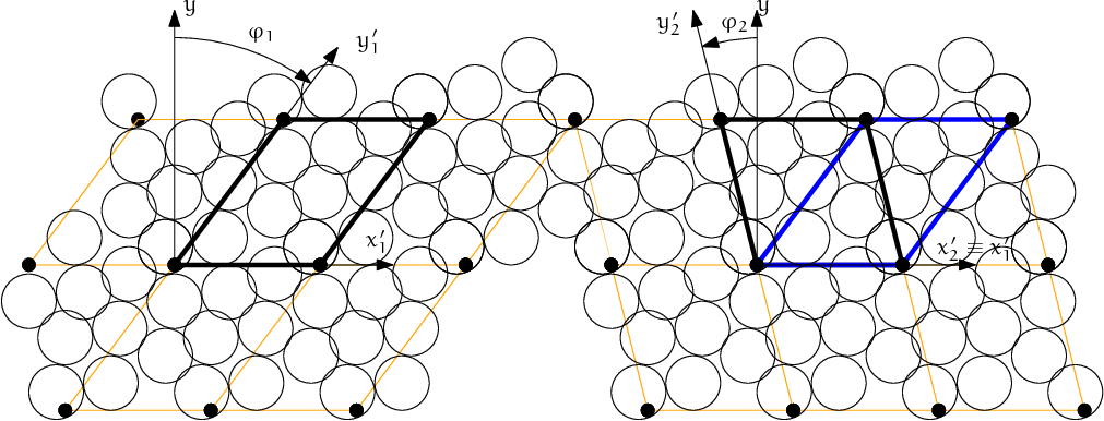
Flipping cell (Cell.flipCell) to avoid infinite stretch of the bounding boxes’ spans with growing $\phi$. Cell flip does not affect interactions from the point of view of the simulation. The periodic arrangement on the left is the same as the one on the right, only the cell is situated differently between identical grid points of repetition; at the same time $|{\phi }_2|<|{\phi }_1|$ and sphere bounding box’s $x$-span stretched by $1/\cos \phi$ becomes smaller. Flipping can be repeated, making effective infinite shear possible.

This algorithm is implemented in InsertionSortCollider and is used whenever simulation is periodic (Omega.isPeriodic); individual BoundFunctor’s are responsible for computing sheared Aabb’s; currently it is implemented for spheres and facets (in Bo1_Sphere_Aabb and Bo1_Facet_Aabb respectively).

Exact collision detection

When the collider detects approximate contact (on the Aabb level) and the contact does not yet exist, it creates potential contact, which is subsequently checked by exact collision algorithms (depending on the combination of Shapes). Since particles can interact over many periodic cells (recall we never change their positions in simulation space), the collider embeds the relative cell coordinate of particles in the interaction itself (Interaction.cellDist) as an integer vector $c$. Multiplying current cell size $\mathit{T}\mathit{s}$ by $c$ component-wise, we obtain particle offset $\mathrm{\Delta }\mathit{x}$ in aperiodic $R^3$; this value is passed (from InteractionLoop) to the functor computing exact collision (IGeomFunctor), which adds it to the position of the particle Interaction.id2.

By storing the integral offset $c$, $\mathrm{\Delta }\mathit{x}$ automatically updates as cell parameters change.

Periodic insertion sort algorithm

The extension of sweep and prune algorithm (described in Sweep and prune) to periodic boundary conditions is non-trivial. Its cornerstone is a periodic variant of the insertion sort algorithm, which involves keeping track of the “period” of each boundary; e.g. taking period $⟨0,10)$, then $8_1\equiv -2_2<2_2$ (subscript indicating period). Doing so efficiently (without shuffling data in memory around as bound wraps from one period to another) requires moving period boundary rather than bounds themselves and making the comparison work transparently at the edge of the container.

This algorithm was also extended to handle non-orthogonal periodic Cell boundaries by working in transformed rather than Cartesian coordinates; this modifies computation of Aabb from Cartesian coordinates in which bodies are positioned (treated in detail in Approximate collision detection).

The sort algorithm is tracking Aabb extrema along all axes. At the collider’s initialization, each value is assigned an integral period, i.e. its distance from the cell’s interior expressed in the cell’s dimension along its respective axis, and is wrapped to a value inside the cell. We put the period number in subscript.

Let us give an example of coordinate sequence along $x$ axis (in a real case, the number of elements would be even, as there is maximum and minimum value couple for each particle; this demonstration only shows the sorting algorithm, however.)

with cell $x$-size $s_x=10$. The $4_1$ value then means that the real coordinate $x_i$ of this extremum is $x_i+1\cdot 10=4$, i.e. $x_i=-4$. The $||$ symbol denotes the periodic cell boundary.

Sorting starts from the first element in the cell, i.e. right of $||$, and inverts elements as in the aperiodic variant. The rules are, however, more complicated due to the presence of the boundary $||$:

($\le$)	stop inverting if neighbors are ordered;
($||\bullet$)	current element left of $||$ is below 0 (lower period boundary); in this case, decrement element’s period, decrease its coordinate by $s_x$ and move $||$ right;
($\bullet ||$)	current element right of $||$ is above $s_x$ (upper period boundary); increment element’s period, increase its coordinate by $s_x$ and move $||$ left;
($||<$)	inversion across $||$ must subtract $s_x$ from the left coordinate during comparison. If the elements are not in order, they are swapped, but they must have their periods changed as they traverse $||$. Apply ($||\circ$) if necessary;
($||\circ$)	if after ($||<$) the element that is now right of $||$ has $x_i<s_x$, decrease its coordinate by $s_x$ and decrement its period. Do not move $||$.

In the first step, ($||\bullet$) is applied, and inversion with ${12}_2$ happens; then we stop because of ($\le$):

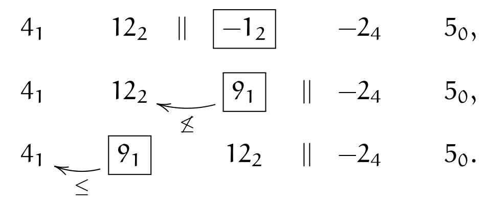
We move to next element $\boxed{-2_4}$; first, we apply ($||\bullet$), then invert until ($\le$):

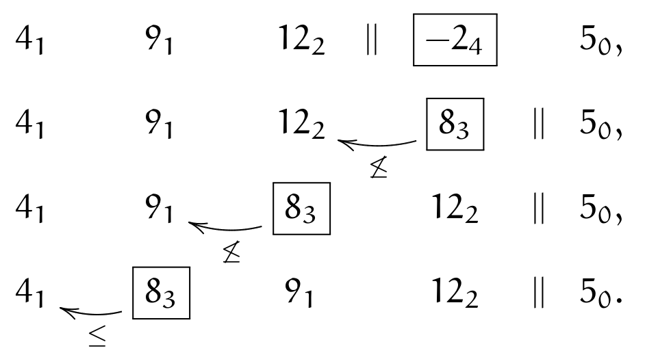
The next element is $\boxed{5_0}$; we satisfy ($||<$), therefore instead of comparing ${12}_2>5_0$, we must do $({12}_2-s_x)=2_3\le 5$; we adjust periods when swapping over $||$ and apply ($||\circ$), turning ${12}_2$ into $2_3$; then we keep inverting, until ($\le$):

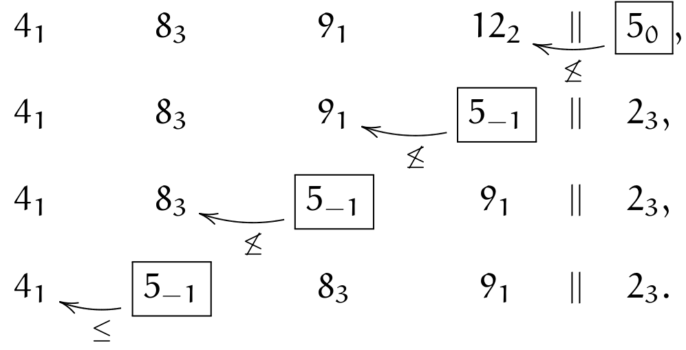
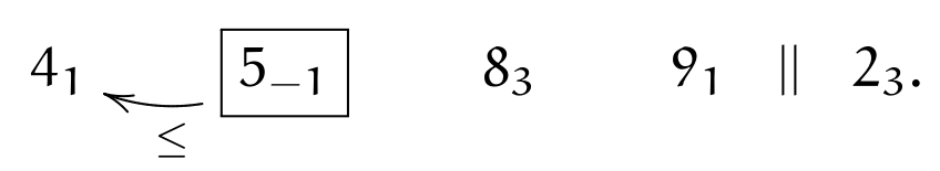
We move (wrapping around) to $\boxed{4_1}$, which is ordered:

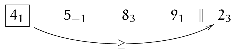
and so is the last element

Computational aspects

Cost

The DEM computation using an explicit integration scheme demands a relatively high number of steps during simulation, compared to implicit scehemes. The total computation time $Z$ of simulation spanning $T$ seconds (of simulated time), containing $N$ particles in volume $V$ depends on:

• linearly, the number of steps $i=T/(s_t\mathrm{\Delta }{t}_{\mathrm{c}\mathrm{r}})$, where $s_t$ is timestep safety factor; $\mathrm{\Delta }{t}_{\mathrm{c}\mathrm{r}}$ can be estimated by p-wave velocity using $E$ and $\rho$ (sect. Estimation of \Dtcr by wave propagation speed) as $\mathrm{\Delta }{t}_{\mathrm{c}\mathrm{r}}^{(p)}=r\sqrt{\frac{\rho }{E}}$. Therefore

  $$i=\frac{T}{s_{t}r}\sqrt{\frac{E}{\rho }}.$$

• the number of particles $N$; for fixed value of simulated domain volume $V$ and particle radius $r$

  $$N=p\frac{V}{\frac{4}{3}\pi r^3},$$

  where $p$ is packing porosity, roughly $\frac{1}{2}$ for dense irregular packings of spheres of similar radius.

  The dependency is not strictly linear (which would be the best case), as some algorithms do not scale linearly; a case in point is the sweep and prune collision detection algorithm introduced in sect. Sweep and prune, with scaling roughly $\mathcal{O}(N\log N)$.

  The number of interactions scales with $N$, as long as packing characteristics are the same.

• the number of computational cores $n_{\mathrm{c}\mathrm{p}\mathrm{u}}$; in the ideal case, the dependency would be inverse-linear were all algorithms parallelized (in Yade, collision detection is not).

Let us suppose linear scaling. Additionally, let us suppose that the material to be simulated ($E$, $\rho$) and the simulation setup ($V$, $T$) are given in advance. Finally, dimensionless constants $s_t$, $p$ and $n_{\mathrm{c}\mathrm{p}\mathrm{u}}$ will have a fixed value. This leaves us with one last degree of freedom, $r$. We may write

$$Z\propto iN\frac{1}{n_{\mathrm{c}\mathrm{p}\mathrm{u}}}=\frac{T}{s_{t}r}\sqrt{\frac{E}{\rho }}p\frac{V}{\frac{4}{3}\pi r^3}\frac{1}{n_{\mathrm{c}\mathrm{p}\mathrm{u}}}\propto \frac{1}{r}\frac{1}{r^3}=\frac{1}{r^4}.$$

This (rather trivial) result is essential to realize DEM scaling; if we want to have finer results, refining the “mesh” by halving $r$, the computation time will grow $2^4=16$ times.

For very crude estimates, one can use a known simulation to obtain a machine “constant”

$$\mu =\frac{Z}{Ni}$$

with the meaning of time per particle and per timestep (in the order of ${10}^{-6}\mathrm{s}$ for current machines). $\mu$ will be only useful if simulation characteristics are similar and non-linearities in scaling do not have major influence, i.e. $N$ should be in the same order of magnitude as in the reference case.

Result indeterminism

It is naturally expected that running the same simulation several times will give exactly the same results: although the computation is done with finite precision, round-off errors would be deterministically the same at every run. While this is true for single-threaded computation where exact order of all operations is given by the simulation itself, it is not true anymore in multi-threaded computation which is described in detail in later sections.

The straight-forward manner of parallel processing in explicit DEM is given by the possibility of treating interactions in arbitrary order. Strain and stress is evaluated for each interaction independently, but forces from interactions have to be summed up. If summation order is also arbitrary (in Yade, forces are accumulated for each thread in the order interactions are processed, then summed together), then the results can be slightly different. For instance

(1/10.)+(1/13.)+(1/17.)=0.23574660633484162
(1/17.)+(1/13.)+(1/10.)=0.23574660633484165

As forces generated by interactions are assigned to bodies in quasi-random order, summary force $F_i$ on the body can be different between single-threaded and multi-threaded computations, but also between different runs of multi-threaded computation with exactly the same parameters. Exact thread scheduling by the kernel is not predictable since it depends on asynchronous events (hardware interrupts) and other unrelated tasks running on the system; and it is thread scheduling that ultimately determines summation order of force contributions from interactions.