User’s manual

Scene construction

Adding particles

The BodyContainer holds Body objects in the simulation; it is accessible as O.bodies.

Creating Body objects

Body objects are only rarely constructed by hand by their components (Shape, Bound, State, Material); instead, convenience functions sphere, facet and wall are used to create them. Using these functions also ensures better future compatibility, if internals of Body change in some way. These functions receive geometry of the particle and several other characteristics. See their documentation for details. If the same Material is used for several (or many) bodies, it can be shared by adding it in O.materials, as explained below.

Defining materials

The O.materials object (instance of Omega.materials) holds defined shared materials for bodies. It only supports addition, and will typically hold only a few instances (though there is no limit).

label given to each material is optional, but can be passed to sphere and other functions for constructing body. The value returned by O.materials.append is an id of the material, which can be also passed to sphere – it is a little bit faster than using label, though not noticeable for small number of particles and perhaps less convenient.

If no Material is specified when calling sphere, the last defined material is used; that is a convenient default. If no material is defined yet (hence there is no last material), a default material will be created: FrictMat(density=1e3,young=1e7,poisson=.3,frictionAngle=.5). This should not happen for serious simulations, but is handy in simple scripts, where exact material properties are more or less irrelevant.

Yade [1]: len(O.materials)
Out[1]: 0

Yade [2]: idConcrete=O.materials.append(FrictMat(young=30e9,poisson=.2,frictionAngle=.6,label="concrete"))

Yade [3]: O.materials[idConcrete]
Out[3]: <FrictMat instance at 0x6184170>

# uses the last defined material
Yade [4]: O.bodies.append(sphere(center=(0,0,0),radius=1))
Out[4]: 0

# material given by id
Yade [5]: O.bodies.append(sphere((0,0,2),1,material=idConcrete))
Out[5]: 1

# material given by label
Yade [6]: O.bodies.append(sphere((0,2,0),1,material="concrete"))
Out[6]: 2

Yade [7]: idSteel=O.materials.append(FrictMat(young=210e9,poisson=.25,frictionAngle=.8,label="steel"))

Yade [8]: len(O.materials)
Out[8]: 2

# implicitly uses "steel" material, as it is the last one now
Yade [9]: O.bodies.append(facet([(1,0,0),(0,1,0),(-1,-1,0)]))
Out[9]: 3

Adding multiple particles

As shown above, bodies are added one by one or several at the same time using the append method:

Yade [10]: O.bodies.append(sphere((0,10,0),1))
Out[10]: 0

Yade [11]: O.bodies.append(sphere((0,0,2),1))
Out[11]: 1

# this is the same, but in one function call
Yade [12]: O.bodies.append([
   ....:   sphere((0,0,0),1),
   ....:   sphere((1,1,3),1)
   ....: ])
   ....: 
Out[12]: [2, 3]

Many functions introduced in next sections return list of bodies which can be readily added to the simulation, including

• packing generators, such as pack.randomDensePack, pack.regularHexa

• surface function pack.gtsSurface2Facets

• import functions ymport.gmsh, ymport.stl, …

As those functions use sphere and facet internally, they accept additional arguments passed to those functions. In particular, material for each body is selected following the rules above (last one if not specified, by label, by index, etc.).

Clumping particles together

In some cases, you might want to create rigid aggregate of individual particles (i.e. particles will retain their mutual position during simulation). This we call a clump. A clump is internally represented by a special body, referenced by clumpId of its members (see also isClump, isClumpMember and isStandalone). Like every body a clump has a position, which is the (mass) balance point between all members. A clump body itself has no interactions with other bodies. Interactions between clumps is represented by interactions between clump members. There are no interactions between clump members of the same clump.

YADE supports different ways of creating clumps:

• Create clumps and spheres (clump members) directly with one command:

The function appendClumped() is designed for this task. For instance, we might add 2 spheres tied together:

Yade [13]: O.bodies.appendClumped([
   ....:    sphere([0,0,0],1),
   ....:    sphere([0,0,2],1)
   ....: ])
   ....: 
Out[13]: (2, [0, 1])

Yade [14]: len(O.bodies)
Out[14]: 3

Yade [15]: O.bodies[1].isClumpMember, O.bodies[2].clumpId
Out[15]: (True, 2)

Yade [16]: O.bodies[2].isClump, O.bodies[2].clumpId
Out[16]: (True, 2)

-> appendClumped() returns a tuple of ids (clumpId,[memberId1,memberId2,...])

• Use existing spheres and clump them together:

For this case the function clump() can be applied on a list of existing bodies:

Yade [17]: bodyList = []

Yade [18]: for ii in range(0,5):
   ....:    bodyList.append(O.bodies.append(sphere([ii,0,1],.5)))#create a "chain" of 5 spheres
   ....: 

Yade [19]: print(bodyList)
[0, 1, 2, 3, 4]

Yade [20]: idClump=O.bodies.clump(bodyList)

-> clump() returns clumpId

• Another option is to replace standalone spheres from a given packing (see SpherePack and makeCloud) by clumps using clump templates.

This is done by a function called replaceByClumps(). This function takes a list of clumpTemplates() and a list of amounts and replaces spheres by clumps. The volume of a new clump will be the same as the volume of the sphere, that was replaced (clump volume/mass/inertia is accounting for overlaps assuming that there are only pair overlaps).

-> replaceByClumps() returns a list of tuples: [(clumpId1,[memberId1,memberId2,...]),(clumpId2,[memberId1,memberId2,...]),...]

It is also possible to add bodies to a clump and release bodies from a clump. Also you can erase the clump (clump members will become standalone).

Additionally YADE allows to achieve the roundness of a clump or roundness coefficient of a packing. Parts of the packing can be excluded from roundness measurement via exclude list.

Yade [21]: bodyList = []

Yade [22]: for ii in range(1,5):
   ....:    bodyList.append(O.bodies.append(sphere([ii,ii,ii],.5)))
   ....: 

Yade [23]: O.bodies.clump(bodyList)
Out[23]: 4

Yade [24]: RC=O.bodies.getRoundness()

Yade [25]: print(RC)
0.25619141423166986

-> getRoundness() returns roundness coefficient RC of a packing or a part of the packing

Note

Have a look at examples/clumps/ folder. There you will find some examples, that show usage of different functions for clumps.

Sphere packings

Representing a solid of an arbitrary shape by arrangement of spheres presents the problem of sphere packing, i.e. spatial arrangement of spheres such that a given solid is approximately filled with them. For the purposes of DEM simulation, there can be several requirements.

1. Distribution of spheres’ radii. Arbitrary volume can be filled completely with spheres provided there are no restrictions on their radius; in such case, number of spheres can be infinite and their radii approach zero. Since both number of particles and minimum sphere radius (via critical timestep) determine computation cost, radius distribution has to be given mandatorily. The most typical distribution is uniform: mean±dispersion; if dispersion is zero, all spheres will have the same radius.

2. Smooth boundary. Some algorithms treat boundaries in such way that spheres are aligned on them, making them smoother as surface.

3. Packing density, or the ratio of spheres volume and solid size. It is closely related to radius distribution.

4. Coordination number, (average) number of contacts per sphere.

5. Isotropy (related to regularity/irregularity); packings with preferred directions are usually not desirable, unless the modeled solid also has such preference.

6. Permissible Spheres’ overlap; some algorithms might create packing where spheres slightly overlap; since overlap usually causes forces in DEM, overlap-free packings are sometimes called “stress-free‟.

Volume representation

There are 2 methods for representing exact volume of the solid in question in Yade: boundary representation and constructive solid geometry. Despite their fundamental differences, they are abstracted in Yade in the Predicate class. Predicate provides the following functionality:

1. defines axis-aligned bounding box for the associated solid (optionally defines oriented bounding box);

2. can decide whether given point is inside or outside the solid; most predicates can also (exactly or approximately) tell whether the point is inside and satisfies some given padding distance from the represented solid boundary (so that sphere of that volume doesn’t stick out of the solid).

Constructive Solid Geometry (CSG)

CSG approach describes volume by geometric primitives or primitive solids (sphere, cylinder, box, cone, …) and boolean operations on them. Primitives defined in Yade include inCylinder, inSphere, inEllipsoid, inHyperboloid, notInNotch.

For instance, hyperboloid (dogbone) specimen for tension-compression test can be constructed in this way (shown at img. img-hyperboloid):

from yade import pack

## construct the predicate first
pred=pack.inHyperboloid(centerBottom=(0,0,-.1),centerTop=(0,0,.1),radius=.05,skirt=.03)
## alternatively: pack.inHyperboloid((0,0,-.1),(0,0,.1),.05,.03)

## pack the predicate with spheres (will be explained later)
spheres=pack.randomDensePack(pred,spheresInCell=2000,radius=3.5e-3)

## add spheres to simulation
O.bodies.append(spheres)

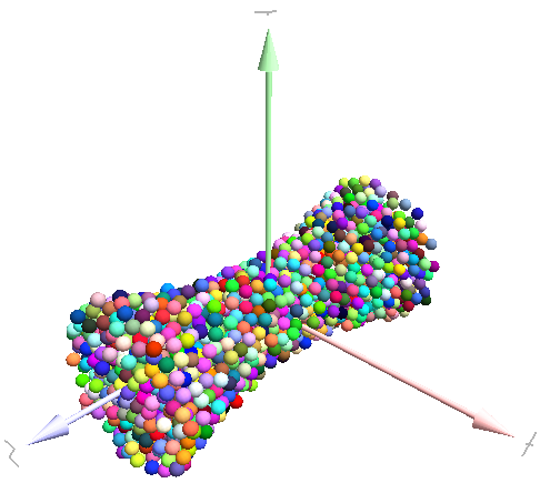
Specimen constructed with the pack.inHyperboloid predicate, packed with pack.randomDensePack.

Boundary representation (BREP)

Representing a solid by its boundary is much more flexible than CSG volumes, but is mostly only approximate. Yade interfaces to GNU Triangulated Surface Library (GTS) to import surfaces readable by GTS, but also to construct them explicitly from within simulation scripts. This makes possible parametric construction of rather complicated shapes; there are functions to create set of 3d polylines from 2d polyline (pack.revolutionSurfaceMeridians), to triangulate surface between such set of 3d polylines (pack.sweptPolylines2gtsSurface).

For example, we can construct a simple funnel (examples/funnel.py, shown at img-funnel):

from numpy import linspace
from yade import pack

# angles for points on circles
thetas=linspace(0,2*pi,num=16,endpoint=True)

# creates list of polylines in 3d from list of 2d projections
# turned from 0 to π
meridians=pack.revolutionSurfaceMeridians(
        [[(3+rad*sin(th),10*rad+rad*cos(th)) for th in thetas] for rad in linspace(1,2,num=10)],
        linspace(0,pi,num=10)
)

# create surface
surf=pack.sweptPolylines2gtsSurface(
        meridians
        +[[Vector3(5*sin(-th),-10+5*cos(-th),30) for th in thetas]]  # add funnel top
)

# add to simulation
O.bodies.append(pack.gtsSurface2Facets(surf))

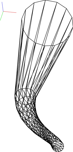
Triangulated funnel, constructed with the examples/funnel.py script.

GTS surface objects can be used for 2 things:

1. pack.gtsSurface2Facets function can create the triangulated surface (from Facet particles) in the simulation itself, as shown in the funnel example. (Triangulated surface can also be imported directly from a STL file using ymport.stl.)

2. pack.inGtsSurface predicate can be created, using the surface as boundary representation of the enclosed volume.

The examples/gts-horse/gts-horse.py (img. img-horse) shows both possibilities; first, a GTS surface is imported:

import gts
surf=gts.read(open('horse.coarse.gts'))

That surface object is used as predicate for packing:

pred=pack.inGtsSurface(surf)
aabb=pred.aabb()
radius=(aabb[1][0]-aabb[0][0])/40
O.bodies.append(pack.regularHexa(pred,radius=radius,gap=radius/4.))

and then, after being translated, as base for triangulated surface in the simulation itself:

surf.translate(0,0,-(aabb[1][2]-aabb[0][2]))
O.bodies.append(pack.gtsSurface2Facets(surf,wire=True))

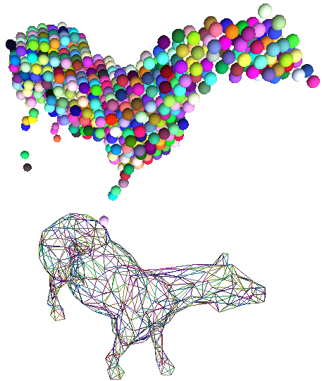
Imported GTS surface (horse) used as packing predicate (top) and surface constructed from facets (bottom). See http://www.youtube.com/watch?v=PZVruIlUX1A for movie of this simulation.

Boolean operations on predicates

Boolean operations on pair of predicates (noted A and B) are defined:

• intersection A & B (conjunction): point must be in both predicates involved.

• union A | B (disjunction): point must be in the first or in the second predicate.

• difference A - B (conjunction with second predicate negated): the point must be in the first predicate and not in the second one.

• symmetric difference A ^ B (exclusive disjunction): point must be in exactly one of the two predicates.

Composed predicates also properly define their bounding box. For example, we can take box and remove cylinder from inside, using the A - B operation (img. img-predicate-difference):

pred=pack.inAlignedBox((-2,-2,-2),(2,2,2))-pack.inCylinder((0,-2,0),(0,2,0),1)
spheres=pack.randomDensePack(pred,spheresInCell=2000,radius=.1,rRelFuzz=.4,returnSpherePack=True)
spheres.toSimulation()

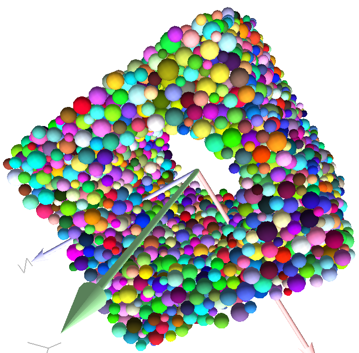
Box with cylinder removed from inside, using difference of these two predicates.

Packing algorithms

Algorithms presented below operate on geometric spheres, defined by their center and radius. With a few exception documented below, the procedure is as follows:

1. Sphere positions and radii are computed (some functions use volume predicate for this, some do not)

2. sphere is called for each position and radius computed; it receives extra keyword arguments of the packing function (i.e. arguments that the packing function doesn’t specify in its definition; they are noted **kw). Each sphere call creates actual Body objects with Sphere shape. List of Body objects is returned.

3. List returned from the packing function can be added to simulation using toSimulation(). Legacy code used a call to O.bodies.append.

Taking the example of pierced box:

pred=pack.inAlignedBox((-2,-2,-2),(2,2,2))-pack.inCylinder((0,-2,0),(0,2,0),1)
spheres=pack.randomDensePack(pred,spheresInCell=2000,radius=.1,rRelFuzz=.4,wire=True,color=(0,0,1),material=1,returnSpherePack=True)

Keyword arguments wire, color and material are not declared in pack.randomDensePack, therefore will be passed to sphere, where they are also documented. spheres is now a SpherePack object.:

spheres.toSimulation()

Packing algorithms described below produce dense packings. If one needs loose packing, SpherePack class provides functions for generating loose packing, via its makeCloud() method. It is used internally for generating initial configuration in dynamic algorithms. For instance:

from yade import pack
sp=pack.SpherePack()
sp.makeCloud(minCorner=(0,0,0),maxCorner=(3,3,3),rMean=.2,rRelFuzz=.5)

will fill given box with spheres, until no more spheres can be placed. The object can be used to add spheres to simulation:

sp.toSimulation()

Geometric

Geometric algorithms compute packing without performing dynamic simulation; among their advantages are

• speed;

• spheres touch exactly, there are no overlaps (what some people call “stress-free” packing);

their chief disadvantage is that radius distribution cannot be prescribed exactly, save in specific cases (regular packings); sphere radii are given by the algorithm, which already makes the system determined. If exact radius distribution is important for your problem, consider dynamic algorithms instead.

Regular

Yade defines packing generators for spheres with constant radii, which can be used with volume predicates as described above. They are dense orthogonal packing (pack.regularOrtho) and dense hexagonal packing (pack.regularHexa). The latter creates so-called “hexagonal close packing”, which achieves maximum density (http://en.wikipedia.org/wiki/Close-packing_of_spheres).

Clear disadvantage of regular packings is that they have very strong directional preferences, which might not be an issue in some cases.

Irregular

Random geometric algorithms do not integrate at all with volume predicates described above; rather, they take their own boundary/volume definition, which is used during sphere positioning. On the other hand, this makes it possible for them to respect boundary in the sense of making spheres touch it at appropriate places, rather than leaving empty space in-between.

GenGeo

is library (python module) for packing generation developed with ESyS-Particle. It creates packing by random insertion of spheres with given radius range. Inserted spheres touch each other exactly and, more importantly, they also touch the boundary, if in its neighbourhood. Boundary is represented as special object of the GenGeo library (Sphere, cylinder, box, convex polyhedron, …). Therefore, GenGeo cannot be used with volume represented by yade predicates as explained above.

Packings generated by this module can be imported directly via ymport.gengeo, or from saved file via ymport.gengeoFile. There is an example script examples/test/genCylLSM.py. Full documentation for GenGeo can be found at ESyS documentation website.

There are debian packages esys-particle and python-demgengeo.

Dynamic

The most versatile algorithm for random dense packing is provided by pack.randomDensePack. Initial loose packing of non-overlapping spheres is generated by randomly placing them in cuboid volume, with radii given by requested (currently only uniform) radius distribution. When no more spheres can be inserted, the packing is compressed and then uncompressed (see py/pack/pack.py for exact values of these “stresses”) by running a DEM simulation; Omega.switchScene is used to not affect existing simulation). Finally, resulting packing is clipped using provided predicate, as explained above.

By its nature, this method might take relatively long; and there are 2 provisions to make the computation time shorter:

• If number of spheres using the spheresInCell parameter is specified, only smaller specimen with periodic boundary is created and then repeated as to fill the predicate. This can provide high-quality packing with low regularity, depending on the spheresInCell parameter (value of several thousands is recommended).

• Providing memoizeDb parameter will make pack.randomDensePack first look into provided file (SQLite database) for packings with similar parameters. On success, the packing is simply read from database and returned. If there is no similar pre-existent packing, normal procedure is run, and the result is saved in the database before being returned, so that subsequent calls with same parameters will return quickly.

If you need to obtain full periodic packing (rather than packing clipped by predicate), you can use pack.randomPeriPack.

In case of specific needs, you can create packing yourself, “by hand”. For instance, packing boundary can be constructed from facets, letting randomly positioned spheres in space fall down under gravity.

Triangulated surfaces

Yade integrates with the the GNU Triangulated Surface library, exposed in python via GTS module. GTS provides variety of functions for surface manipulation (coarsening, tesselation, simplification, import), to be found in its documentation.

GTS surfaces are geometrical objects, which can be inserted into simulation as set of particles whose Body.shape is of type Facet – single triangulation elements. pack.gtsSurface2Facets can be used to convert GTS surface triangulation into list of bodies ready to be inserted into simulation via O.bodies.append.

Facet particles are created by default as non-Body.dynamic (they have zero inertial mass). That means that they are fixed in space and will not move if subject to forces. You can however

• prescribe arbitrary movement to facets using a PartialEngine (such as TranslationEngine or RotationEngine);

• assign explicitly mass and inertia to that particle;

• make that particle part of a clump and assign mass and inertia of the clump itself (described below).

Note

Facets can only (currently) interact with spheres, not with other facets, even if they are dynamic. Collision of 2 facets will not create interaction, therefore no forces on facets.

Import

Yade currently offers 3 formats for importing triangulated surfaces from external files, in the ymport module:

ymport.gts

text file in native GTS format.

ymport.stl

STereoLitography format, in either text or binary form; exported from Blender, but from many CAD systems as well.

ymport.gmsh.

text file in native format for GMSH, popular open-source meshing program.

If you need to manipulate surfaces before creating list of facets, you can study the py/ymport.py file where the import functions are defined. They are rather simple in most cases.

Parametric construction

The GTS module provides convenient way of creating surface by vertices, edges and triangles.

Frequently, though, the surface can be conveniently described as surface between polylines in space. For instance, cylinder is surface between two polygons (closed polylines). The pack.sweptPolylines2gtsSurface offers the functionality of connecting several polylines with triangulation.

Note

The implementation of pack.sweptPolylines2gtsSurface is rather simplistic: all polylines must be of the same length, and they are connected with triangles between points following their indices within each polyline (not by distance). On the other hand, points can be co-incident, if the threshold parameter is positive: degenerate triangles with vertices closer that threshold are automatically eliminated.

Manipulating lists efficiently (in terms of code length) requires being familiar with list comprehensions in python.

Another examples can be found in examples/mill.py (fully parametrized) or examples/funnel.py (with hardcoded numbers).

Creating interactions

In typical cases, interactions are created during simulations as particles collide. This is done by a Collider detecting approximate contact between particles and then an IGeomFunctor detecting exact collision.

Some material models (such as the concrete model) rely on initial interaction network which is denser than geometrical contact of spheres: sphere’s radii as “enlarged” by a dimensionless factor called interaction radius (or interaction ratio) to create this initial network. This is done typically in this way (see examples/concrete/uniax.py for an example):

1. Approximate collision detection is adjusted so that approximate contacts are detected also between particles within the interaction radius. This consists in setting value of Bo1_Sphere_Aabb.aabbEnlargeFactor to the interaction radius value.

2. The geometry functor (Ig2) would normally say that “there is no contact” if given 2 spheres that are not in contact. Therefore, the same value as for Bo1_Sphere_Aabb.aabbEnlargeFactor must be given to it (Ig2_Sphere_Sphere_ScGeom.interactionDetectionFactor ).

   Note that only Sphere + Sphere interactions are supported; there is no parameter analogous to distFactor in Ig2_Facet_Sphere_ScGeom. This is on purpose, since the interaction radius is meaningful in bulk material represented by sphere packing, whereas facets usually represent boundary conditions which should be exempt from this dense interaction network.

3. Run one single step of the simulation so that the initial network is created.

4. Reset interaction radius in both Bo1 and Ig2 functors to their default value again.

5. Continue the simulation; interactions that are already established will not be deleted (the Law2 functor in use permitting).

In code, such scenario might look similar to this one (labeling is explained in Labeling things):

intRadius=1.5
damping=0.05

O.engines=[
   ForceResetter(),
   InsertionSortCollider([
      # enlarge here
      Bo1_Sphere_Aabb(aabbEnlargeFactor=intRadius,label='bo1s'),
      Bo1_Facet_Aabb(),
        ]),
   InteractionLoop(
      [
         # enlarge here
         Ig2_Sphere_Sphere_ScGeom(interactionDetectionFactor=intRadius,label='ig2ss'),
         Ig2_Facet_Sphere_ScGeom(),
      ],
      [Ip2_CpmMat_CpmMat_CpmPhys()],
      [Law2_ScGeom_CpmPhys_Cpm(epsSoft=0)], # deactivated
   ),
   NewtonIntegrator(damping=damping,label='damper'),
]

# run one single step
O.step()

# reset interaction radius to the default value
bo1s.aabbEnlargeFactor=1.0
ig2ss.interactionDetectionFactor=1.0

# now continue simulation
O.run()

Individual interactions on demand

It is possible to create an interaction between a pair of particles independently of collision detection using createInteraction. This function looks for and uses matching Ig2 and Ip2 functors. Interaction will be created regardless of distance between given particles (by passing a special parameter to the Ig2 functor to force creation of the interaction even without any geometrical contact). Appropriate constitutive law should be used to avoid deletion of the interaction at the next simulation step.

Yade [26]: O.materials.append(FrictMat(young=3e10,poisson=.2,density=1000))
Out[26]: 0

Yade [27]: O.bodies.append([
   ....:    sphere([0,0,0],1),
   ....:    sphere([0,0,1000],1)
   ....: ])
   ....: 
Out[27]: [0, 1]

# only add InteractionLoop, no other engines are needed now
Yade [28]: O.engines=[
   ....:    InteractionLoop(
   ....:        [Ig2_Sphere_Sphere_ScGeom(),],
   ....:        [Ip2_FrictMat_FrictMat_FrictPhys()],
   ....:        [] # not needed now
   ....:    )
   ....: ]
   ....: 

Yade [29]: i=createInteraction(0,1)

# created by functors in InteractionLoop
Yade [30]: i.geom, i.phys
Out[30]: (<ScGeom instance at 0x618c880>, <FrictPhys instance at 0x6110570>)

This method will be rather slow if many interactions are to be created (the functor lookup will be repeated for each of them). In such case, ask on yade-dev@lists.launchpad.net to have the createInteraction function accept list of pairs id’s as well.

Assigning cohesive bonds (possibly between distant bodies)

A particular case of interactions on demand is when cohesive strength needs to be assigned to interactions when using Law2_ScGeom6D_CohFrictPhys_CohesionMoment.

• For existing interactions, it can be done using setCohesion. If physFunctor is physics functor of type Ip2_CohFrictMat_CohFrictMat_CohFrictPhys and i an existing, cohesionless, interaction, this line would assign cohesion without changing the current contact force/moments:

  physFunctor.setCohesion(i,cohesive=True,resetDisp=False)
  

• For creating new interactions (particularly when the interaction needs to be created between distant bodies), the interaction needs to be created, first, then cohesion can be assigned:

  i=createInteraction(i.id1,i.id2)
  physFunctor.setCohesion(i,cohesive=True,resetDisp=False)
  

If the above lines are executed between distant bodies, the interaction will be initially in traction. In order to make it force free we need to use current distance as equilibrium distance, this is achieved with resetDisp=True.

• Creating cohesive bonds with this method between many thousand of distant bodies can be a challenge since it needs to identify the candidate pairs. In such situation, it is suggested to exploit the collision detection engine to establish the list of close - though distant - neighbours. Indeed, the collider can be executed outside the time-integration loop, with a user-defined detection distance, in order to produce that list. This technique is examplified in examples/cohesion/assignCohesionRemote.py.

Base engines

A typical DEM simulation in Yade does at least the following at each step (see Function components for details):

1. Reset forces from previous step

2. Detect new collisions

3. Handle interactions

4. Apply forces and update positions of particles

Each of these points corresponds to one or several engines:

O.engines=[
   ForceResetter(),          # reset forces
   InsertionSortCollider([...]),  # approximate collision detection
   InteractionLoop([...],[...],[...]) # handle interactions
   NewtonIntegrator()        # apply forces and update positions
]

The order of engines is important. In majority of cases, you will put any additional engine after InteractionLoop:

• if it applies force, it should come before NewtonIntegrator, otherwise the force will never be effective.

• if it makes use of bodies’ positions, it should also come before NewtonIntegrator, otherwise, positions at the next step will be used (this might not be critical in many cases, such as output for visualization with VTKRecorder).

The O.engines sequence must be always assigned at once (the reason is in the fact that although engines themselves are passed by reference, the sequence is copied from c++ to Python or from Python to c++). This includes modifying an existing O.engines; therefore

O.engines.append(SomeEngine()) # wrong

will not work;

O.engines=O.engines+[SomeEngine()] # ok

must be used instead. For inserting an engine after position #2 (for example), use python slice notation:

O.engines=O.engines[:2]+[SomeEngine()]+O.engines[2:]

Note

When Yade starts, O.engines is filled with a reasonable default list, so that it is not strictly necessary to redefine it when trying simple things. The default scene will handle spheres, boxes, and facets with frictional properties correctly, and adjusts the timestep dynamically. You can find an example in examples/simple-scene/simple-scene-default-engines.py.

Functors choice

In the above example, we omited functors, only writing ellipses ... instead. As explained in Dispatchers and functors, there are 4 kinds of functors and associated dispatchers. User can choose which ones to use, though the choice must be consistent.

Bo1 functors

Bo1 functors must be chosen depending on the collider in use; they are given directly to the collider (which internally uses BoundDispatcher).

At this moment (January 2019), the most common choice is InsertionSortCollider, which uses Aabb; functors creating Aabb must be used in that case. Depending on particle shapes in your simulation, choose appropriate functors:

O.engines=[...,
   InsertionSortCollider([Bo1_Sphere_Aabb(),Bo1_Facet_Aabb()]),
   ...
]

Using more functors than necessary (such as Bo1_Facet_Aabb if there are no facets in the simulation) has no performance penalty. On the other hand, missing functors for existing shapes will cause those bodies to not collide with other bodies (they will freely interpenetrate).

There are other colliders as well, though their usage is only experimental:

• SpatialQuickSortCollider is correctness-reference collider operating on Aabb; it is significantly slower than InsertionSortCollider.

• PersistentTriangulationCollider only works on spheres; it does not use a BoundDispatcher, as it operates on spheres directly.

• FlatGridCollider is proof-of-concept grid-based collider, which computes grid positions internally (no BoundDispatcher either)

Ig2 functors

Ig2 functor choice (all of them derive from IGeomFunctor) depends on

1. shape combinations that should collide; for instance:

   InteractionLoop([Ig2_Sphere_Sphere_ScGeom()],[],[])
   

   will handle collisions for Sphere + Sphere, but not for Facet + Sphere – if that is desired, an additional functor must be used:

   InteractionLoop([
      Ig2_Sphere_Sphere_ScGeom(),
      Ig2_Facet_Sphere_ScGeom()
   ],[],[])
   

   Again, missing combination will cause given shape combinations to freely interpenetrate one another. There are several possible choices of a functor for each pair, hence they cannot be put into InsertionSortCollider by default. A common mistake for bodies going through each other is that the necessary functor was not added.

2. IGeom type accepted by the Law2 functor (below); it is the first part of functor’s name after Law2 (for instance, Law2_ScGeom_CpmPhys_Cpm accepts ScGeom).

Ip2 functors

Ip2 functors (deriving from IPhysFunctor) must be chosen depending on

1. Material combinations within the simulation. In most cases, Ip2 functors handle 2 instances of the same Material class (such as Ip2_FrictMat_FrictMat_FrictPhys for 2 bodies with FrictMat)

2. IPhys accepted by the constitutive law (Law2 functor), which is the second part of the Law2 functor’s name (e.g. Law2_ScGeom_FrictPhys_CundallStrack accepts FrictPhys)

Note

Unlike with Bo1 and Ig2 functors, unhandled combination of Materials is an error condition signaled by an exception.

Law2 functor(s)

Law2 functor was the ultimate criterion for the choice of Ig2 and Ip2 functors; there are no restrictions on its choice in itself, as it only applies forces without creating new objects.

In most simulations, only one Law2 functor will be in use; it is possible, though, to have several of them, dispatched based on combination of IGeom and IPhys produced previously by Ig2 and Ip2 functors respectively (in turn based on combination of Shapes and Materials).

Note

As in the case of Ip2 functors, receiving a combination of IGeom and IPhys which is not handled by any Law2 functor is an error.

Warning

Many Law2 exist in Yade, and new ones can appear at any time. In some cases different functors are only different implementations of the same contact law (e.g. Law2_ScGeom_FrictPhys_CundallStrack and Law2_L3Geom_FrictPhys_ElPerfPl). Also, sometimes, the peculiarity of one functor may be reproduced as a special case of a more general one. Therefore, for a given constitutive behavior, the user may have the choice between different functors. It is strongly recommended to favor the most used and most validated implementation when facing such choice. A list of available functors classified from mature to unmaintained is updated here to guide this choice.

Examples

Let us give several examples of the chain of created and accepted types.

Basic DEM model

Suppose we want to use the Law2_ScGeom_FrictPhys_CundallStrack constitutive law. We see that

1. the Ig2 functors must create ScGeom. If we have for instance spheres and boxes in the simulation, we will need functors accepting Sphere + Sphere and Box + Sphere combinations. We don’t want interactions between boxes themselves (as a matter of fact, there is no such functor anyway). That gives us Ig2_Sphere_Sphere_ScGeom and Ig2_Box_Sphere_ScGeom.

2. the Ip2 functors should create FrictPhys. Looking at InteractionPhysicsFunctors, there is only Ip2_FrictMat_FrictMat_FrictPhys. That obliges us to use FrictMat for particles.

The result will be therefore:

InteractionLoop(
   [Ig2_Sphere_Sphere_ScGeom(),Ig2_Box_Sphere_ScGeom()],
   [Ip2_FrictMat_FrictMat_FrictPhys()],
   [Law2_ScGeom_FrictPhys_CundallStrack()]
)

Concrete model

In this case, our goal is to use the Law2_ScGeom_CpmPhys_Cpm constitutive law.

• We use spheres and facets in the simulation, which selects Ig2 functors accepting those types and producing ScGeom: Ig2_Sphere_Sphere_ScGeom and Ig2_Facet_Sphere_ScGeom.

• We have to use Material which can be used for creating CpmPhys. We find that CpmPhys is only created by Ip2_CpmMat_CpmMat_CpmPhys, which determines the choice of CpmMat for all particles.

Therefore, we will use:

InteractionLoop(
   [Ig2_Sphere_Sphere_ScGeom(),Ig2_Facet_Sphere_ScGeom()],
   [Ip2_CpmMat_CpmMat_CpmPhys()],
   [Law2_ScGeom_CpmPhys_Cpm()]
)

Imposing conditions

In most simulations, it is not desired that all particles float freely in space. There are several ways of imposing boundary conditions that block movement of all or some particles with regard to global space.

Note

When using Clump bodies discussed in above section Clumping particles together, the following paragraphs apply to the Clump bodies themselves (not to their members).

Motion constraints

• Body.dynamic determines whether a body will be accelerated by NewtonIntegrator; it is mandatory to make it false for bodies with zero mass, where applying non-zero force would result in infinite displacement.

  Facets are case in the point: facet makes them non-dynamic by default, as they have zero volume and zero mass (this can be changed, by passing dynamic=True to facet or setting Body.dynamic; setting State.mass to a non-zero value must be done as well). The same is true for wall.

  Making sphere non-dynamic is achieved simply by:

  b = sphere([x,y,z],radius,dynamic=False)
  b.dynamic=True #revert the previous
  

• State.blockedDOFs permits selective blocking of any of 6 degrees of freedom in global space. For instance, a sphere can be made to move only in the xy plane by saying:

  Yade [31]: O.bodies.append(sphere((0,0,0),1))
  Out[31]: 0
  
  Yade [32]: O.bodies[0].state.blockedDOFs='zXY'
  

  In contrast to Body.dynamic, blockedDOFs will only block forces (and acceleration) in selected directions. Actually, b.dynamic=False is nearly only a shorthand for b.state.blockedDOFs=='xyzXYZ' . A subtle difference is that the former does reset the velocity components automaticaly, while the latest does not. If you prescribed linear or angular velocity, they will be applied regardless of blockedDOFs. It also implies that if the velocity is not zero when degrees of freedom are blocked via blockedDOFs assignements, the body will keep moving at the velocity it has at the time of blocking. The differences are shown below:

  Yade [33]: b1 = sphere([0,0,0],1,dynamic=True)
  
  Yade [34]: b1.state.blockedDOFs
  Out[34]: ''
  
  Yade [35]: b1.state.vel = Vector3(1,0,0) #we want it to move...
  
  Yade [36]: b1.dynamic = False #... at a constant velocity
  
  Yade [37]: print(b1.state.blockedDOFs, b1.state.vel)
  xyzXYZ Vector3(0,0,0)
  
  Yade [38]: # oops, velocity has been reset when setting dynamic=False
  
  Yade [39]: b1.state.vel = (1,0,0) # we can still assign it now
  
  Yade [40]: print(b1.state.blockedDOFs, b1.state.vel)
  xyzXYZ Vector3(1,0,0)
  
  Yade [41]: b2 = sphere([0,0,0],1,dynamic=True) #another try
  
  Yade [42]: b2.state.vel = (1,0,0)
  
  Yade [43]: b2.state.blockedDOFs = "xyzXYZ" #this time we assign blockedDOFs directly, velocity is unchanged
  
  Yade [44]: print(b2.state.blockedDOFs, b2.state.vel)
  xyzXYZ Vector3(1,0,0)
  

It might be desirable to constrain motion of some particles constructed from a generated sphere packing, following some condition, such as being at the bottom of a specimen; this can be done by looping over all bodies with a conditional:

for b in O.bodies:
   # block all particles with z coord below .5:
   if b.state.pos[2]<.5: b.dynamic=False

Arbitrary spatial predicates introduced above can be expoited here as well:

from yade import pack
pred=pack.inAlignedBox(lowerCorner,upperCorner)
for b in O.bodies:
   if not isinstance(b.shape,Sphere): continue # skip non-spheres
   # ask the predicate if we are inside
   if pred(b.state.pos,b.shape.radius): b.dynamic=False

Imposing motion and forces

Imposed velocity

If a degree of freedom is blocked and a velocity is assigned along that direction (translational or rotational velocity), then the body will move at constant velocity. This is the simpler and recommended method to impose the motion of a body. This, for instance, will result in a constant velocity along \(x\) (it can still be freely accelerated along \(y\) and \(z\)):

O.bodies.append(sphere((0,0,0),1))
O.bodies[0].state.blockedDOFs='x'
O.bodies[0].state.vel=(10,0,0)

Conversely, modifying the position directly is likely to break Yade’s algorithms, especially those related to collision detection and contact laws, as they are based on bodies velocities. Therefore, unless you really know what you are doing, don’t do that for imposing a motion:

O.bodies.append(sphere((0,0,0),1))
O.bodies[0].state.blockedDOFs='x'
O.bodies[0].state.pos=10*O.dt #REALLY BAD! Don't assign position

Imposed force

Applying a force or a torque on a body is done via functions of the ForceContainer. It is as simple as this:

O.forces.addF(0,(1,0,0)) #applies for one step

This way, the force applies for one time step only, and is resetted at the beginning of each step. For this reason, imposing a force at the begining of one step will have no effect at all, since it will be immediatly resetted. The only way is to place a PyRunner inside the simulation loop.

Applying the force permanently is possible with another function (in this case it does not matter if the command comes at the begining of the time step):

O.forces.setPermF(0,(1,0,0)) #applies permanently

The force will persist across iterations, until it is overwritten by another call to O.forces.setPermF(id,f) or erased by O.forces.reset(resetAll=True). The permanent force on a body can be checked with O.forces.permF(id).

Boundary controllers

Engines deriving from BoundaryController impose boundary conditions during simulation, either directly, or by influencing several bodies. You are referred to their individual documentation for details, though you might find interesting in particular

• UniaxialStrainer for applying strain along one axis at constant rate; useful for plotting strain-stress diagrams for uniaxial loading case. See examples/concrete/uniax.py for an example.

• TriaxialStressController which applies prescribed stress/strain along 3 perpendicular axes on cuboid-shaped packing using 6 walls (Box objects)

• PeriTriaxController for applying stress/strain along 3 axes independently, for simulations using periodic boundary conditions (Cell)

Field appliers

Engines deriving from FieldApplier are acting on all particles. The one most used is GravityEngine applying uniform acceleration field (GravityEngine is deprecated, use NewtonIntegrator.gravity instead).

Partial engines

Engines deriving from PartialEngine define the ids attribute determining bodies which will be affected. Several of them warrant explicit mention here:

• TranslationEngine and RotationEngine for applying constant speed linear and rotational motion on subscribers.

• ForceEngine and TorqueEngine applying given values of force/torque on subscribed bodies at every step.

• StepDisplacer for applying generalized displacement delta at every timestep; designed for precise control of motion when testing constitutive laws on 2 particles.

The real value of partial engines is when you need to prescribe a complex type of force or displacement field. For moving a body at constant velocity or for imposing a single force, the methods explained in Imposing motion and forces are much simpler. There are several interpolating engines (InterpolatingDirectedForceEngine for applying force with varying magnitude, InterpolatingHelixEngine for applying spiral displacement with varying angular velocity; see examples/test/helix.py and possibly others); writing a new interpolating engine is rather simple using examples of those that already exist.

Convenience features

Labeling things

Engines and functors can define a label attribute. Whenever the O.engines sequence is modified, python variables of those names are created/updated; since it happens in the __builtins__ namespaces, these names are immediately accessible from anywhere. This was used in Creating interactions to change interaction radius in multiple functors at once.

Warning

Make sure you do not use label that will overwrite (or shadow) an object that you already use under that variable name. Take care not to use syntactically wrong names, such as “er*452” or “my engine”; only variable names permissible in Python can be used.

Simulation tags

Omega.tags is a dictionary (it behaves like a dictionary, although the implementation in C++ is different) mapping keys to labels. Contrary to regular python dictionaries that you could create,

• O.tags is saved and loaded with simulation;

• O.tags has some values pre-initialized.

After Yade startup, O.tags contains the following:

Yade [45]: dict(O.tags) # convert to real dictionary
Out[45]: 
{'author': 'root~(root@runner-bgledujk-project-10133144-concurrent-0)',
 'isoTime': '20241114T041932',
 'id': '20241114T041932p37',
 'd.id': '20241114T041932p37',
 'id.d': '20241114T041932p37'}

author

Real name, username and machine as obtained from your system at simulation creation

id

Unique identifier of this Yade instance (or of the instance which created a loaded simulation). It is composed of date, time and process number. Useful if you run simulations in parallel and want to avoid overwriting each other’s outputs; embed O.tags['id'] in output filenames (either as directory name, or as part of the file’s name itself) to avoid it. This is explained in Separating output files from jobs in detail.

isoTime

Time when simulation was created (with second resolution).

d.id, id.d

Simulation description and id joined by period (and vice-versa). Description is used in batch jobs; in non-batch jobs, these tags are identical to id.

You can add your own tags by simply assigning value, with the restriction that the left-hand side object must be a string and must not contain =.

Yade [46]: O.tags['anythingThat I lik3']='whatever'

Yade [47]: O.tags['anythingThat I lik3']
Out[47]: 'whatever'

Saving python variables

Python variable lifetime is limited; in particular, if you save simulation, variables will be lost after reloading. Yade provides limited support for data persistence for this reason (internally, it uses special values of O.tags). The functions in question are saveVars and loadVars.

saveVars takes dictionary (variable names and their values) and a mark (identification string for the variable set); it saves the dictionary inside the simulation. These variables can be re-created (after the simulation was loaded from a XML file, for instance) in the yade.params.mark namespace by calling loadVars with the same identification mark:

Yade [48]: a=45; b=pi/3

Yade [49]: saveVars('ab',a=a,b=b)

# save simulation (we could save to disk just as well)
Yade [49]: O.saveTmp()

Yade [51]: O.loadTmp()

Yade [52]: loadVars('ab')

Yade [53]: yade.params.ab.a
Out[53]: 45

# import like this
Yade [54]: from yade.params import ab

Yade [55]: ab.a, ab.b
Out[55]: (45, 1.0471975511965976)

# also possible
Yade [56]: from yade.params import *

Yade [57]: ab.a, ab.b
Out[57]: (45, 1.0471975511965976)

Enumeration of variables can be tedious if they are many; creating local scope (which is a function definition in Python, for instance) can help:

def setGeomVars():
        radius=4
        thickness=22
        p_t=4/3*pi
        dim=Vector3(1.23,2.2,3)
        #
        # define as much as you want here
        # it all appears in locals() (and nothing else does)
        #
        saveVars('geom',loadNow=True,**locals())

setGeomVars()
from yade.params.geom import *
# use the variables now

Note

Only types that can be pickled can be passed to saveVars.

Controlling simulation

Tracking variables

Running python code

A special engine PyRunner can be used to periodically call python code, specified via the command parameter. Periodicity can be controlled by specifying computation time (realPeriod), virtual time (virtPeriod) or iteration number (iterPeriod).

For instance, to print kinetic energy (using kineticEnergy) every 5 seconds, the following engine will be put to O.engines:

PyRunner(command="print('kinetic energy',kineticEnergy())",realPeriod=5)

For running more complex commands, it is convenient to define an external function and only call it from within the engine. Since the command is run in the script’s namespace, functions defined within scripts can be called. Let us print information on interaction between bodies 0 and 1 periodically:

def intrInfo(id1,id2):
        try:
                i=O.interactions[id1,id2]
                # assuming it is a CpmPhys instance
                print (d1,id2,i.phys.sigmaN)
        except:
                # in case the interaction doesn't exist (yet?)
                print("No interaction between",id1,id2)
O.engines=[...,
        PyRunner(command="intrInfo(0,1)",realPeriod=5)
]

Warning

If a function was declared inside a live yade session (ipython) then an error NameError: name 'intrInfo' is not defined will occur unless python globals() are updated with command

globals().update(locals())

More useful examples will be given below.

The plot module provides simple interface and storage for tracking various data. Although originally conceived for plotting only, it is widely used for tracking variables in general.

The data are in plot.data dictionary, which maps variable names to list of their values; the plot.addData function is used to add them.

Yade [58]: from yade import plot

Yade [59]: plot.data
Out[59]: {}

Yade [60]: plot.addData(sigma=12,eps=1e-4)

# not adding sigma will add a NaN automatically
# this assures all variables have the same number of records
Yade [61]: plot.addData(eps=1e-3)

# adds NaNs to already existing sigma and eps columns
Yade [62]: plot.addData(force=1e3)

Yade [63]: plot.data
Out[63]: 
{'sigma': [12, nan, nan],
 'eps': [0.0001, 0.001, nan],
 'force': [nan, nan, 1000.0]}

# retrieve only one column
Yade [64]: plot.data['eps']
Out[64]: [0.0001, 0.001, nan]

# get maximum eps
Yade [65]: max(plot.data['eps'])
Out[65]: 0.001

New record is added to all columns at every time plot.addData is called; this assures that lines in different columns always match. The special value nan or NaN (Not a Number) is inserted to mark the record invalid.

Note

It is not possible to have two columns with the same name, since data are stored as a dictionary.

To record data periodically, use PyRunner. This will record the z coordinate and velocity of body #1, iteration number and simulation time (every 20 iterations):

O.engines=O.engines+[PyRunner(command='myAddData()', iterPeriod=20)]

from yade import plot
def myAddData():
        b=O.bodies[1]
        plot.addData(z1=b.state.pos[2], v1=b.state.vel.norm(), i=O.iter, t=O.time)

Note

Arbitrary string can be used as a column label for plot.data. However if the name has spaces inside (e.g. my funny column) or is a reserved python keyword (e.g. for) the only way to pass it to plot.addData is to use a dictionary:

plot.addData(**{'my funny column':1e3, 'for':0.3})

An exception are columns having leading of trailing whitespaces. They are handled specially in plot.plots and should not be used (see below).

Labels can be conveniently used to access engines in the myAddData function:

O.engines=[...,
        UniaxialStrainer(...,label='strainer')
]
def myAddData():
        plot.addData(sigma=strainer.avgStress,eps=strainer.strain)

In that case, naturally, the labeled object must define attributes which are used (UniaxialStrainer.strain and UniaxialStrainer.avgStress in this case).

Plotting variables

Above, we explained how to track variables by storing them using plot.addData. These data can be readily used for plotting. Yade provides a simple, quick to use, plotting in the plot module. Naturally, since direct access to underlying data is possible via plot.data, these data can be processed in any other way.

The plot.plots dictionary is a simple specification of plots. Keys are x-axis variable, and values are tuple of y-axis variables, given as strings that were used for plot.addData; each entry in the dictionary represents a separate figure:

plot.plots={
        'i':('t',),     # plot t(i)
        't':('z1','v1') # z1(t) and v1(t)
}

Actual plot using data in plot.data and plot specification of plot.plots can be triggered by invoking the plot.plot function.

Live updates of plots

Yade features live-updates of figures during calculations. It is controlled by following settings:

• plot.live - By setting yade.plot.live=True you can watch the plot being updated while the calculations run. Set to False otherwise.

• plot.liveInterval - This is the interval in seconds between the plot updates.

• plot.autozoom - When set to True the plot will be automatically rezoomed.

Controlling line properties

In this subsection let us use a basic complete script like examples/simple-scene/simple-scene-plot.py, which we will later modify to make the plots prettier. Line of interest from that file is, and generates a picture presented below:

plot.plots={'i':('t'),'t':('z_sph',None,('v_sph','go-'),'z_sph_half')}

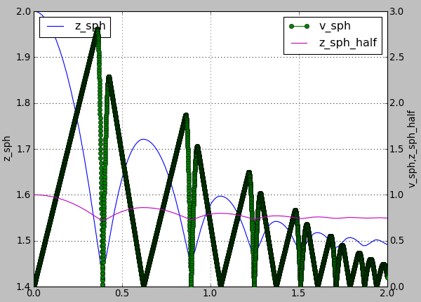
Figure generated by examples/simple-scene/simple-scene-plot.py.

The line plots take an optional second string argument composed of a line color (eg. 'r', 'g' or 'b'), a line style (eg. '-', '–-' or ':') and a line marker ('o', 's' or 'd'). A red dotted line with circle markers is created with ‘ro:’ argument. For a listing of all options please have a look at http://matplotlib.sourceforge.net/api/pyplot_api.html#matplotlib.pyplot.plot

For example using following plot.plots() command, will produce a following graph:

plot.plots={'i':(('t','xr:'),),'t':(('z_sph','r:'),None,('v_sph','g--'),('z_sph_half','b-.'))}

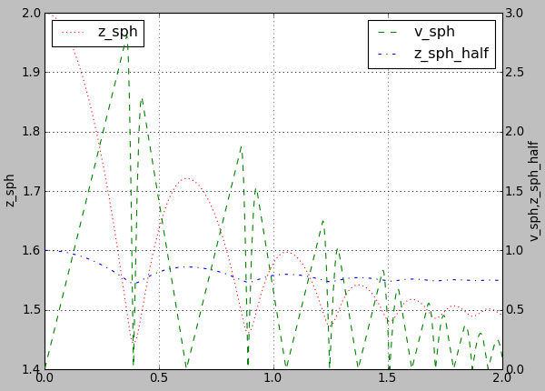
Figure generated by changing parameters to plot.plots as above.

And this one will produce a following graph:

plot.plots={'i':(('t','xr:'),),'t':(('z_sph','Hr:'),None,('v_sph','+g--'),('z_sph_half','*b-.'))}

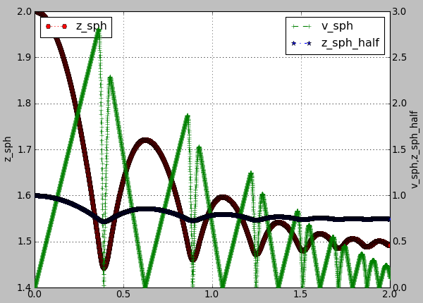
Figure generated by changing parameters to plot.plots as above.

Note

You can learn more in matplotlib tutorial http://matplotlib.sourceforge.net/users/pyplot_tutorial.html and documentation http://matplotlib.sourceforge.net/users/pyplot_tutorial.html#controlling-line-properties

Note

Please note that there is an extra , in 'i':(('t','xr:'),), otherwise the 'xr:' wouldn’t be recognized as a line style parameter, but would be treated as an extra data to plot.

Controlling text labels

It is possible to use TeX syntax in plot labels. For example using following two lines in examples/simple-scene/simple-scene-plot.py, will produce a following picture:

plot.plots={'i':(('t','xr:'),),'t':(('z_sph','r:'),None,('v_sph','g--'),('z_sph_half','b-.'))}
plot.labels={'z_sph':'$z_{sph}$' , 'v_sph':'$v_{sph}$' , 'z_sph_half':'$z_{sph}/2$'}

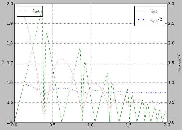
Figure generated by examples/simple-scene/simple-scene-plot.py, with TeX labels.

Greek letters are simply a '$\alpha$', '$\beta$' etc. in those labels. To change the font style a following command could be used:

yade.plot.matplotlib.rc('mathtext', fontset='stixsans')

But this is not part of yade, but a part of matplotlib, and if you want something more complex you really should have a look at matplotlib users manual http://matplotlib.sourceforge.net/users/index.html

Multiple figures

Since plot.plots is a dictionary, multiple entries with the same key (x-axis variable) would not be possible, since they overwrite each other:

Yade [66]: plot.plots={
   ....:    'i':('t',),
   ....:    'i':('z1','v1')
   ....: }
   ....: 

Yade [67]: plot.plots
Out[67]: {'i': ('z1', 'v1')}

You can, however, distinguish them by prepending/appending space to the x-axis variable, which will be removed automatically when looking for the variable in plot.data – both \(x\)-axes will use the i column:

Yade [68]: plot.plots={
   ....:    'i':('t',),
   ....:    'i ':('z1','v1') # note the space in 'i '
   ....: }
   ....: 

Yade [69]: plot.plots
Out[69]: {'i': ('t',), 'i ': ('z1', 'v1')}

Split y1 y2 axes

To avoid big range differences on the \(y\) axis, it is possible to have left and right \(y\) axes separate (like axes x1y2 in gnuplot). This is achieved by inserting None to the plot specifier; variables coming before will be plot normally (on the left y-axis), while those after will appear on the right:

plot.plots={'i':('z1',None,'v1')}

Exporting

Plots and data can be exported to external files for later post-processing in Gnuplot via that plot.saveGnuplot function. Note that all data you added via plot.addData is saved - even data that you don’t plot live during simulation. By editing the generated .gnuplot file you can plot any of the added Data afterwards.

• Data file is saved (compressed using bzip2) separately from the gnuplot file, so any other programs can be used to process them. In particular, the numpy.genfromtxt (documented here) can be useful to import those data back to python; the decompression happens automatically.

• The gnuplot file can be run through gnuplot to produce the figure; see plot.saveGnuplot documentation for details.

For post-processing with other tools than gnuplot, saved data can also be exported in another kind of text file with plot.saveDataTxt.

Stop conditions

For simulations with a pre-determined number of steps, it can be prescribed:

# absolute iteration number
O.stopAtIter=35466
O.run()
O.wait()

or

# number of iterations to run from now
O.run(35466,True) # wait=True

causes the simulation to run 35466 iterations, then stopping.

Frequently, decisions have to be made based on evolution of the simulation itself, which is not yet known. In such case, a function checking some specific condition is called periodically; if the condition is satisfied, O.pause or other functions can be called to stop the stimulation. See documentation for Omega.run, Omega.pause, Omega.step, Omega.stopAtIter for details.

For simulations that seek static equilibrium, the unbalancedForce can provide a useful metrics (see its documentation for details); for a desired value of 1e-2 or less, for instance, we can use:

def checkUnbalanced():
        if unbalancedForce<1e-2: O.pause()

O.engines=O.engines+[PyRunner(command="checkUnbalanced()",iterPeriod=100)]

# this would work as well, without the function defined apart:
#   PyRunner(command="if unablancedForce<1e-2: O.pause()",iterPeriod=100)

O.run(); O.wait()
# will continue after O.pause() will have been called

Arbitrary functions can be periodically checked, and they can also use history of variables tracked via plot.addData. For example, this is a simplified version of damage control in examples/concrete/uniax.py; it stops when current stress is lower than half of the peak stress:

O.engines=[...,
        UniaxialStrainer=(...,label='strainer'),
        PyRunner(command='myAddData()',iterPeriod=100),
        PyRunner(command='stopIfDamaged()',iterPeriod=100)
]

def myAddData():
        plot.addData(t=O.time,eps=strainer.strain,sigma=strainer.stress)

def stopIfDamaged():
        currSig=plot.data['sigma'][-1] # last sigma value
        maxSig=max(plot.data['sigma']) # maximum sigma value
        # print something in any case, so that we know what is happening
        print(plot.data['eps'][-1],currSig)
        if currSig<.5*maxSig:
                print("Damaged, stopping")
                print('gnuplot',plot.saveGnuplot(O.tags['id']))
                import sys
                sys.exit(0)

O.run(); O.wait()
# this place is never reached, since we call sys.exit(0) directly

Checkpoints

Occasionally, it is useful to revert to simulation at some past point and continue from it with different parameters. For instance, tension/compression test will use the same initial state but load it in 2 different directions. Two functions, Omega.saveTmp and Omega.loadTmp are provided for this purpose; memory is used as storage medium, which means that saving is faster, and also that the simulation will disappear when Yade finishes.

O.saveTmp()
# do something
O.saveTmp('foo')
O.loadTmp()      # loads the first state
O.loadTmp('foo') # loads the second state

Warning

O.loadTmp cannot be called from inside an engine, since before loading a simulation, the old one must finish the current iteration; it would lead to deadlock, since O.loadTmp would wait for the current iteration to finish, while the current iteration would be blocked on O.loadTmp.

A special trick must be used: a separate function to be run after the current iteration is defined and is invoked from an independent thread launched only for that purpose:

O.engines=[...,PyRunner('myFunc()',iterPeriod=345)]

def myFunc():
        if someCondition:
                import thread
                # the () are arguments passed to the function
                thread.start_new_thread(afterIterFunc,())
def afterIterFunc():
        O.pause(); O.wait() # wait till the iteration really finishes
        O.loadTmp()

O.saveTmp()
O.run()

Remote control

Yade can be controlled remotely over network. At yade startup, the following lines appear, among other messages:

TCP python prompt on localhost:9000, auth cookie `dcekyu'
TCP info provider on localhost:21000

They inform about 2 ports on which connection of 2 different kind is accepted.

Python prompt

TCP python prompt is telnet server with authenticated connection, providing full python command-line. It listens on port 9000, or higher if already occupied (by another yade instance, for example).

Using the authentication cookie, connection can be made using telnet:

$ telnet localhost 9000
Trying 127.0.0.1...
Connected to localhost.
Escape character is '^]'.
Enter auth cookie: dcekyu
__   __    ____                 __  _____ ____ ____
\ \ / /_ _|  _ \  ___    ___   / / |_   _/ ___|  _ \
 \ V / _` | | | |/ _ \  / _ \ / /    | || |   | |_) |
  | | (_| | |_| |  __/ | (_) / /     | || |___|  __/
  |_|\__,_|____/ \___|  \___/_/      |_| \____|_|

(connected from 127.0.0.1:40372)
>>>

The python pseudo-prompt >>> lets you write commands to manipulate simulation in variety of ways as usual. Two things to notice:

1. The new python interpreter (>>>) lives in a namespace separate from Yade [1]: command-line. For your convenience, from yade import * is run in the new python instance first, but local and global variables are not accessible (only builtins are).

2. The (fake) >>> interpreter does not have rich interactive feature of IPython, which handles the usual command-line Yade [1]:; therefore, you will have no command history, ? help and so on.

Note

By giving access to python interpreter, full control of the system (including reading user’s files) is possible. For this reason, connection is only allowed from localhost, not over network remotely. Of course you can log into the system via SSH over network to get remote access.

Warning

Authentication cookie is trivial to crack via bruteforce attack. Although the listener stalls for 5 seconds after every failed login attempt (and disconnects), the cookie could be guessed by trial-and-error during very long simulations on a shared computer.

Info provider

TCP Info provider listens at port 21000 (or higher) and returns some basic information about current simulation upon connection; the connection terminates immediately afterwards. The information is python dictionary represented as string (serialized) using standard pickle module.

This functionality is used by the batch system (described below) to be informed about individual simulation progress and estimated times. If you want to access this information yourself, you can study core/main/yade-batch.in for details.

Batch queuing and execution (yade-batch)

Yade features light-weight system for running one simulation with different parameters; it handles assignment of parameter values to python variables in simulation script, scheduling jobs based on number of available and required cores and more. The whole batch consists of 2 files:

simulation script

regular Yade script, which calls readParamsFromTable to obtain parameters from parameter table. In order to make the script runnable outside the batch, readParamsFromTable takes default values of parameters, which might be overridden from the parameter table.

readParamsFromTable knows which parameter file and which line to read by inspecting the PARAM_TABLE environment variable, set by the batch system.

parameter table

simple text file, each line representing one parameter set. This file is read by readParamsFromTable (using TableParamReader class), called from simulation script, as explained above. For better reading of the text file you can make use of tabulators, these will be ignored by readParamsFromTable. Parameters are not restricted to numerical values. You can also make use of strings by "quoting" them (' ' may also be used instead of " "). This can be useful for nominal parameters.

The batch can be run as

yade-batch parameters.table simulation.py

and it will intelligently run one simulation for each parameter table line. A minimal example is found in examples/test/batch/params.table and examples/test/batch/sim.py, another example follows.

Example

Suppose we want to study influence of parameters density and initialVelocity on position of a sphere falling on fixed box. We create parameter table like this:

description density initialVelocity # first non-empty line are column headings
reference   2400    10
hi_v           =    20              # = to use value from previous line
lo_v           =     5
# comments are allowed
hi_rho      5000    10
# blank lines as well:

hi_rho_v       =    20
hi_rh0_lo_v    =     5

Each line give one combination of these 2 parameters and assigns (which is optional) a description of this simulation.

In the simulation file, we read parameters from table, at the beginning of the script; each parameter has default value, which is used if not specified in the parameters file:

readParamsFromTable(
        gravity=-9.81,
        density=2400,
        initialVelocity=20,
        noTableOk=True     # use default values if not run in batch
)
from yade.params.table import *
print(gravity, density, initialVelocity)

after the call to readParamsFromTable, corresponding python variables are created in the yade.params.table module and can be readily used in the script, e.g.

GravityEngine(gravity=(0,0,gravity))

Let us see what happens when running the batch:

$ yade-batch batch.table batch.py
Will run `/usr/local/bin/yade-trunk' on `batch.py' with nice value 10, output redirected to `batch.@.log', 4 jobs at a time.
Will use table `batch.table', with available lines 2, 3, 4, 5, 6, 7.
Will use lines  2 (reference), 3 (hi_v), 4 (lo_v), 5 (hi_rho), 6 (hi_rho_v), 7 (hi_rh0_lo_v).
Master process pid 7030

These lines inform us about general batch information: nice level, log file names, how many cores will be used (4); table name, and line numbers that contain parameters; finally, which lines will be used; master PID is useful for killing (stopping) the whole batch with the kill command.

Job summary:
   #0 (reference/4): PARAM_TABLE=batch.table:2 DISPLAY=  /usr/local/bin/yade-trunk --threads=4 --nice=10 -x batch.py > batch.reference.log 2>&1
   #1 (hi_v/4): PARAM_TABLE=batch.table:3 DISPLAY=  /usr/local/bin/yade-trunk --threads=4 --nice=10 -x batch.py > batch.hi_v.log 2>&1
   #2 (lo_v/4): PARAM_TABLE=batch.table:4 DISPLAY=  /usr/local/bin/yade-trunk --threads=4 --nice=10 -x batch.py > batch.lo_v.log 2>&1
   #3 (hi_rho/4): PARAM_TABLE=batch.table:5 DISPLAY=  /usr/local/bin/yade-trunk --threads=4 --nice=10 -x batch.py > batch.hi_rho.log 2>&1
   #4 (hi_rho_v/4): PARAM_TABLE=batch.table:6 DISPLAY=  /usr/local/bin/yade-trunk --threads=4 --nice=10 -x batch.py > batch.hi_rho_v.log 2>&1
   #5 (hi_rh0_lo_v/4): PARAM_TABLE=batch.table:7 DISPLAY=  /usr/local/bin/yade-trunk --threads=4 --nice=10 -x batch.py > batch.hi_rh0_lo_v.log 2>&1

displays all jobs with command-lines that will be run for each of them. At this moment, the batch starts to be run.

#0 (reference/4) started on Tue Apr 13 13:59:32 2010
#0 (reference/4) done    (exit status 0), duration 00:00:01, log batch.reference.log
#1 (hi_v/4) started on Tue Apr 13 13:59:34 2010
#1 (hi_v/4) done    (exit status 0), duration 00:00:01, log batch.hi_v.log
#2 (lo_v/4) started on Tue Apr 13 13:59:35 2010
#2 (lo_v/4) done    (exit status 0), duration 00:00:01, log batch.lo_v.log
#3 (hi_rho/4) started on Tue Apr 13 13:59:37 2010
#3 (hi_rho/4) done    (exit status 0), duration 00:00:01, log batch.hi_rho.log
#4 (hi_rho_v/4) started on Tue Apr 13 13:59:38 2010
#4 (hi_rho_v/4) done    (exit status 0), duration 00:00:01, log batch.hi_rho_v.log
#5 (hi_rh0_lo_v/4) started on Tue Apr 13 13:59:40 2010
#5 (hi_rh0_lo_v/4) done    (exit status 0), duration 00:00:01, log batch.hi_rh0_lo_v.log

information about job status changes is being printed, until:

All jobs finished, total time  00:00:08
Log files:
batch.reference.log batch.hi_v.log batch.lo_v.log batch.hi_rho.log batch.hi_rho_v.log batch.hi_rh0_lo_v.log
Bye.

Separating output files from jobs

As one might output data to external files during simulation (using classes such as VTKRecorder), it is important to name files in such way that they are not overwritten by next (or concurrent) job in the same batch. A special tag O.tags['id'] is provided for such purposes: it is comprised of date, time and PID, which makes it always unique (e.g. 20100413T144723p7625); additional advantage is that alphabetical order of the id tag is also chronological. To add the used parameter set or the description of the job, if set, you could add O.tags[‘params’] to the filename.

For smaller simulations, prepending all output file names with O.tags['id'] can be sufficient:

saveGnuplot(O.tags['id'])

For larger simulations, it is advisable to create separate directory of that name first, putting all files inside afterwards:

os.mkdir(O.tags['id'])
O.engines=[
        # …
        VTKRecorder(fileName=O.tags['id']+'/'+'vtk'),
        # …
]
# …
O.saveGnuplot(O.tags['id']+'/'+'graph1')

Controlling parallel computation

Default total number of available cores is determined from /proc/cpuinfo (provided by Linux kernel); in addition, if OMP_NUM_THREADS environment variable is set, minimum of these two is taken. The -j/--jobs option can be used to override this number.

By default, each job uses all available cores for itself, which causes jobs to be effectively run in parallel. Number of cores per job can be globally changed via the --job-threads option.

Table column named !OMP_NUM_THREADS (! prepended to column generally means to assign environment variable, rather than python variable) controls number of threads for each job separately, if it exists.

If number of cores for a job exceeds total number of cores, warning is issued and only the total number of cores is used instead.

Merging gnuplot from individual jobs

Frequently, it is desirable to obtain single figure for all jobs in the batch, for comparison purposes. Somewhat heuristic way for this functionality is provided by the batch system. yade-batch must be run with the --gnuplot option, specifying some file name that will be used for the merged figure:

yade-trunk --gnuplot merged.gnuplot batch.table batch.py

Data are collected in usual way during the simulation (using plot.addData) and saved to gnuplot file via plot.saveGnuplot (it creates 2 files: gnuplot command file and compressed data file). The batch system scans, once the job is finished, log file for line of the form gnuplot [something]. Therefore, in order to print this magic line we put:

print('gnuplot',plot.saveGnuplot(O.tags['id']))

and the end of the script (even after waitIfBatch()) , which prints:

gnuplot 20100413T144723p7625.gnuplot

to the output (redirected to log file).

This file itself contains single graph:

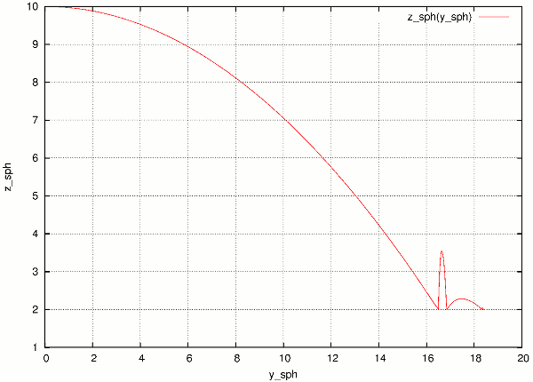
Figure from single job in the batch.

At the end, the batch system knows about all gnuplot files and tries to merge them together, by assembling the merged.gnuplot file.

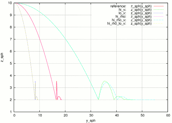
Merged figure from all jobs in the batch. Note that labels are prepended by job description to make lines distinguishable.

HTTP overview

While job is running, the batch system presents progress via simple HTTP server running at port 9080, which can be acessed from a regular web browser (or e.g. lynx for a terminal usage) by requesting the http://localhost:9080 URL. This page can be accessed remotely over network as well.

Summary page available at port 9080 as batch is processed (updates every 5 seconds automatically). Possible job statuses are pending, running, done, failed.

Batch execution on Job-based clusters (OAR)

On High Performance Computation (HPC) clusters with a scheduling system, the following script might be useful. Exactly like yade-batch, it handles assignemnt of parameters value to python variables in simulation script from a parameter table, and job submission. This script is written for oar-based system , and may be extended to others ones. On those system, usually, a job can’t run forever and has a specific duration allocation. The whole job submission consists of 3 files:

Simulation script:

Regular Yade script, which calls readParamsFromTable to obtain parameters from parameter table. In order to make the script runnable outside the batch, readParamsFromTable takes default values of parameters, which might be overridden from the parameter table.

readParamsFromTable knows which parameter file and which line to read by inspecting the PARAM_TABLE environment variable, set by the batch system.

Parameter table:

Simple text file, each line representing one parameter set. This file is read by readParamsFromTable (using TableParamReader class), called from simulation script, as explained above. For better reading of the text file you can make use of tabulators, these will be ignored by readParamsFromTable. Parameters are not restricted to numerical values. You can also make use of strings by "quoting" them ('  ' may also be used instead of "  "). This can be useful for nominal parameters.

Job script:

Bash script, which calls yade on computing nodes. This script eventually creates temp folders, save data to storage server etc. The script must be formatted as a template where some tags will be replaced by specific values at the execution time:

• __YADE_COMMAND__ will be replaced by the actual yade run command

• __YADE_LOGFILE__ will be replaced by the log file path (output to stdout)

• __YADE_ERRFILE__ will be replaced by the error file path (output to stderr)

• __YADE_JOBNO__ will be replaced by an identifier composed as (launch script pid)-(job order)

• __YADE_JOBID__ will be replaced by an identifier composed of all parameters values

The batch can be run as

yade-oar --oar-project=<your project name> --oar-script=job.sh --oar-walltime=hh:mm:ss parameters.table simulation.py

and it will generate one launch script and submit one job for each parameter table line. A minimal example is found in examples/oar/params.table examples/oar/job.sh and examples/oar/sim.py.

Note

You have to specify either –oar-walltime or a !WALLTIME column in params.table. !WALLTIME will override –oar-walltime

Warning

yade-oar is not compiled by default, use -DENABLE_OAR=1 option to cmake to enable it. Please note also that submitting yade jobs (or yade-batch jobs) through OAR does not actually require to use yade-oar. The point of yade-oar is about making yade submit a batch of OAR jobs, instead of sumbitting a yade batch as one OAR job. Mind that it may be viewed as a hack of the OAR scheduler itself by some HPC admins.

Postprocessing

3d rendering & videos

3D rendering is available at runtime to inspect the simulation, it uses QGLViewer library.

Many parameters of the rendering can be modified. See for instance background color bgColor in OpenGLRenderer - also visible in the “Display” tab of Qt Controller, and the keys listed in QGLViewer’s help (hit “h” when the 3D window is active). For instance, hit “t” to switch between orthographic / perspective camera, or “m” to move particle around with the mouse.

colorStyle helps to quickly switch between predefined styles for particle color, background color, and resolution of sphere representation. For images to be included in documents it is generally better to use a white background:

colorStyle.setStyle("figureColor",True)  # colorful particles on white background
colorStyle.setStyle("figureGrey",True)  # grey levels for everything

These two styles also have higher resolution for displaying the spheres. The style that was used pre-2024 is old. The available styles are listed in colorStyle.styles:

Yade [70]: colorStyle.styles
Out[70]: 
{'sand': <yade.utils.YadeColorStyle at 0x7f1a946a4650>,
 'old': <yade.utils.YadeColorStyle at 0x7f1a958fb710>,
 'figureColor': <yade.utils.YadeColorStyle at 0x7f1a94735040>,
 'figureGrey': <yade.utils.YadeColorStyle at 0x7f1a947cb5f0>,
 'blue': <yade.utils.YadeColorStyle at 0x7f1a943b4c20>,
 'screenDisplayLowRes': <yade.utils.YadeColorStyle at 0x7f1a943b4c50>}

3D rendering is one of several ways to produce videos of simulations:

1. Capture screen output (the 3d rendering window) during the simulation − there are tools available for that (such as Istanbul or RecordMyDesktop, which are also packaged for most Linux distributions). The output is “what you see is what you get”, with all the advantages and disadvantages.

2. Periodic frame snapshot using SnapshotEngine (see examples/test/force-network-video.py, examples/bulldozer/bulldozer.py or examples/test/beam-l6geom.py for a complete example):

   O.engines=[
     #...
     SnapshotEngine(iterPeriod=100,fileBase='/tmp/bulldozer-',viewNo=0,label='snapshooter')
   ]
   

   which will save numbered files like /tmp/bulldozer-0000.png. These files can be processed externally (with mencoder and similar tools) or directly with the makeVideo:

   makeVideo(frameSpec,out,renameNotOverwrite=True,fps=24,kbps=6000,bps=None)
   

   The video is encoded using the default mencoder codec (mpeg4).

3. Specialized post-processing tools, notably Paraview. This is described in more detail in the following section.

Paraview

Saving data during the simulation

Paraview is based on the Visualization Toolkit, which defines formats for saving various types of data. One of them (with the .vtu extension) can be written by a special engine VTKRecorder. It is added to the simulation loop:

O.engines=[
        # ...
        VTKRecorder(iterPeriod=100,recorders=['spheres','facets','colors'],fileName='/tmp/p1-')
]

• iterPeriod determines how often to save simulation data (besides iterPeriod, you can also use virtPeriod or realPeriod). If the period is too high (and data are saved only few times), the video will have few frames.

• fileName is the prefix for files being saved. In this case, output files will be named /tmp/p1-spheres.0.vtu and /tmp/p1-facets.0.vtu, where the number is the number of iteration; many files are created, putting them in a separate directory is advisable.

• recorders determines what data to save

export.VTKExporter plays a similar role, with the difference that it is more flexible. It will save any user defined variable associated to the bodies.

Loading data into Paraview

All sets of files (spheres, facets, …) must be opened one-by-one in Paraview. The open dialogue automatically collapses numbered files in one, making it easy to select all of them:

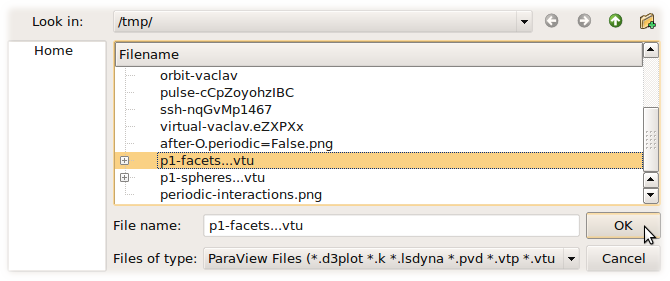
Click on the “Apply” button in the “Object inspector” sub-window to make loaded objects visible. You can see tree of displayed objects in the “Pipeline browser”:

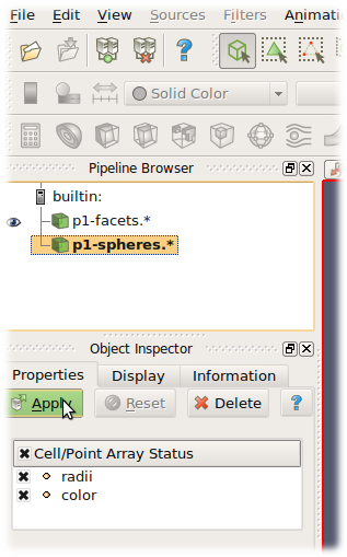
Rendering spherical particles. Glyphs

Spheres will only appear as points. To make them look as spheres, you have to add “glyph” to the p1-spheres.* item in the pipeline using the icon. Then set (in the Object inspector)

• “Glyph type” to Sphere

• “Radius” to 1

• “Scale mode” to Scalar (Scalar is set above to be the radii value saved in the file, therefore spheres with radius 1 will be scaled by their true radius)

• “Set scale factor” to 1

• optionally uncheck “Mask points” and “Random mode” (they make some particles not to be rendered for performance reasons, controlled by the “Maximum Number of Points”)

After clicking “Apply”, spheres will appear. They will be rendered over the original white points, which you can disable by clicking on the eye icon next to p1-spheres.* in the Pipeline browser.

Rendering spherical particles. PointSprite

Another opportunity to display spheres is by using PointSprite plugin. This technique requires much less RAM in comparison to Glyphs.

• “Tools -> Manage Plugins”

• “PointSprite_Plugin -> Load selected -> Close”

• Load VTU-files

• “Representation -> Point Sprite”

• “Point Sprite -> Scale By -> radii”

• “Edit Radius Transfer Function -> Proportional -> Multiplier = 1.0 -> Close”

Rendering interactions as force chain

Data saved by VTKRecorder (the steps below generates cones rather than tubes) or export.VTKExporter(...).exportInteractions(what=dict(forceN='i.phys.normalForce.norm()')) (the steps below generates per interaction tubes with constant radius):

• Load interactions VTP or VTK files

• Filters -> Cell Data To Point Data

• Filters -> Tube

• Set color by “forceN”

• Set “Vary Radius” to “By Scalar”

• Set “Radius” and “Radius Factor” such that the result looks OK (in 3D postprocessing tutorial script, Radius=0.0005 and Radius Factor=100 looks reasonably)

Facet transparency

If you want to make facet objects transparent, select p1-facets.* in the Pipeline browser, then go to the Object inspector on the Display tab. Under “Style”, you can set the “Opacity” value to something smaller than 1.

Animation

You can move between frames (snapshots that were saved) via the “Animation” menu. After setting the view angle, zoom etc to your satisfaction, the animation can be saved with File/Save animation.

Micro-stress and micro-strain

It is sometimes useful to visualize a DEM simulation through equivalent strain fields or stress fields. This is possible with TesselationWrapper. This class handles the triangulation of spheres in a scene, build tesselation on request, and give access to computed quantities: volume, porosity and local deformation for each sphere. The definition of microstrain and microstress is at the scale of particle-centered subdomains shown below, as explained in [Catalano2014a] .

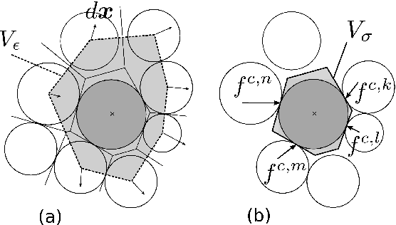
Micro-strain

Below is an output of the defToVtk function visualized with paraview (in this case Yade’s TesselationWrapper was used to process experimental data obtained on sand by Edward Ando at Grenoble University, 3SR lab.). The output is visualized with paraview, as explained in the previous section. Similar results can be generated from simulations:

tt=TriaxialTest()
tt.generate("test.yade")
O.load("test.yade")
O.run(100,True)
TW=TesselationWrapper()
TW.triangulate()        #compute regular Delaunay triangulation, don’t construct tesselation
TW.computeVolumes()     #will silently tesselate the packing, then compute volume of each Voronoi cell
TW.volume(10)           #get volume associated to sphere of id 10
TW.setState(0)          #store current positions internaly for later use as the "0" state
O.run(100,True)         #make particles move a little (let's hope they will!)
TW.setState(1)          #store current positions internaly in the "1" (deformed) state
#Now we can define strain by comparing states 0 and 1, and average them at the particles scale
TW.defToVtk("strain.vtk")

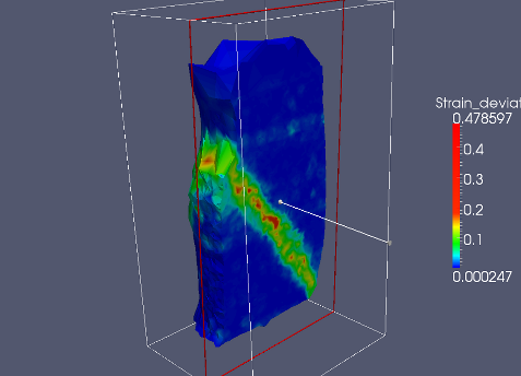
Micro-stress

Stress fields can be generated by combining the volume returned by TesselationWrapper to per-particle stress given by bodyStressTensors. Since the stress \(\sigma\) from bodyStressTensor implies a division by the volume \(V_b\) of the solid particle, one has to re-normalize it in order to obtain the micro-stress as defined in [Catalano2014a] (equation 39 therein), i.e. \(\overline{\sigma}^k = \sigma^k \times V_b^k / V_{\sigma}^k\) where \(V_{\sigma}^k\) is the volume assigned to particle \(k\) in the tesselation. For instance:

#"b" being a body
TW=TesselationWrapper()
TW.setState()
TW.computeVolumes()
s=bodyStressTensors()
stress = s[b.id]*4.*pi/3.*b.shape.radius**3/TW.volume(b.id)

As any other value, the stress can be exported to a vtk file for display in Paraview using export.VTKExporter.

Python specialties and tricks

Importing Yade in other Python applications

Yade can be imported in other Python applications. To do so, you need somehow to make yade executable .py extended. The easiest way is to create a symbolic link, i.e. (suppose your Yade executable file is called “yade-trunk” and you want make it “yadeimport.py”):

$ cd /path/where/you/want/yadeimport
$ ln -s /path/to/yade/executable/yade-trunk yadeimport.py

Then you need to make your yadeimport.py findable by Python. You can export PYTHONPATH environment variable, or simply use sys.path directly in Python script:

import sys
sys.path.append('/path/where/you/want/yadeimport')
from yadeimport import *

print(Matrix3(1,2,3, 4,5,6, 7,8,9))
print(O.bodies)
# any other Yade code

Extending Yade

• new particle shape

• new constitutive law

Troubleshooting

Crashes

It is possible that you encounter crash of Yade, i.e. Yade terminates with error message such as

Segmentation fault (core dumped)

without further explanation. Frequent causes of such conditions are

• program error in Yade itself;

• fatal condition in your particular simulation (such as impossible dispatch);

• problem with graphics card driver.

Try to reproduce the error (run the same script) with debug-enabled version of Yade. Debugger will be automatically launched at crash, showing backtrace of the code (in this case, we triggered crash by hand):

Yade [1]: import os,signal
Yade [2]: os.kill(os.getpid(),signal.SIGSEGV)
SIGSEGV/SIGABRT handler called; gdb batch file is `/tmp/yade-YwtfRY/tmp-0'
GNU gdb (GDB) 7.1-ubuntu
Copyright (C) 2010 Free Software Foundation, Inc.
License GPLv3+: GNU GPL version 3 or later <http://gnu.org/licenses/gpl.html>
This is free software: you are free to change and redistribute it.
There is NO WARRANTY, to the extent permitted by law.  Type "show copying"
and "show warranty" for details.
This GDB was configured as "x86_64-linux-gnu".
For bug reporting instructions, please see:
<http://www.gnu.org/software/gdb/bugs/>.
[Thread debugging using libthread_db enabled]
[New Thread 0x7f0fb1268710 (LWP 16471)]
[New Thread 0x7f0fb29f2710 (LWP 16470)]
[New Thread 0x7f0fb31f3710 (LWP 16469)]

…

What looks as cryptic message is valuable information for developers to locate source of the bug. In particular, there is (usually) line <signal handler called>; lines below it are source of the bug (at least very likely so):

Thread 1 (Thread 0x7f0fcee53700 (LWP 16465)):
#0  0x00007f0fcd8f4f7d in __libc_waitpid (pid=16497, stat_loc=<value optimized out>, options=0) at ../sysdeps/unix/sysv/linux/waitpid.c:41
#1  0x00007f0fcd88c7e9 in do_system (line=<value optimized out>) at ../sysdeps/posix/system.c:149
#2  0x00007f0fcd88cb20 in __libc_system (line=<value optimized out>) at ../sysdeps/posix/system.c:190
#3  0x00007f0fcd0b4b23 in crashHandler (sig=11) at core/main/pyboot.cpp:45
#4  <signal handler called>
#5  0x00007f0fcd87ed57 in kill () at ../sysdeps/unix/syscall-template.S:82
#6  0x000000000051336d in posix_kill (self=<value optimized out>, args=<value optimized out>) at ../Modules/posixmodule.c:4046
#7  0x00000000004a7c5e in call_function (f=Frame 0x1c54620, for file <ipython console>, line 1, in <module> (), throwflag=<value optimized out>) at ../Python/ceval.c:3750
#8  PyEval_EvalFrameEx (f=Frame 0x1c54620, for file <ipython console>, line 1, in <module> (), throwflag=<value optimized out>) at ../Python/ceval.c:2412

If you think this might be error in Yade, file a bug report as explained below. Do not forget to attach full yade output from terminal, including startup messages and debugger output – select with right mouse button, with middle button paste the bugreport to a file and attach it. Attach your simulation script as well.

Reporting bugs

Bugs are general name for defects (functionality shortcomings, misdocumentation, crashes) or feature requests. They are tracked at https://gitlab.com/yade-dev/trunk/issues.

When reporting a new bug, be as specific as possible; state version of yade you use, system version and the output of printAllVersions(), as explained in the above section on crashes.

Getting in touch with Yade community

Public questions and answers for getting help

Hint

Please use the GitLab interface for asking questions about Yade.

In case you’re not familiar with computer oriented discussion lists, please read this wiki page (a Yade-oriented and shortened version of How To Ask Questions The Smart Way) before posting, in order to increase your chances getting help. Do not forget to state what version of Yade you use (shown when you start Yade, or even better as printed by function libVersions.printAllVersions), whether you installed it from source code or a package, what operating system (such as Ubuntu 18.04), and if you have done any local modifications to source code in case of compiled version.

Mailing lists

In addition to the Q&A Launchpad interface, Yade has two mailing-lists. Both are hosted at http://www.launchpad.net and before posting, you must register to Launchpad and subscribe to the list by adding yourself to “team” of the same name running the list.

yade-users@lists.launchpad.net

is a general discussion list for all Yade users. Add yourself to yade-users team so that you can post messages. List archives:

• https://lists.launchpad.net/yade-users/

• http://www.mail-archive.com/yade-users@lists.launchpad.net/

yade-dev@lists.launchpad.net

is for discussions about Yade development; you must be member of yade-dev team to post. This list is archived in two places:

• https://lists.launchpad.net/yade-dev/

• http://www.mail-archive.com/yade-dev@lists.launchpad.net/

Private and/or paid support

You might contact developers by their private email (rather than by the Launchpad interface or the mailing lists) or the generic adress consult|A|yade-dem.org for a closer, private, support. This is also a suitable method for proposing financial reward for implementation of a substantial feature that is not yet in Yade – typically, though, we will request this feature to be part of the public codebase once completed, so that the rest of the community can benefit from it as well.

Wiki

http://www.yade-dem.org/wiki/

Discord chat

https://discord.gg/rku35YXZJd

Twitter account

https://twitter.com/YadeDEM